7.2 Solutions
library(tidyverse)7.2.1 Question 1
Begin by examining summary statistics of the variables age, yrsarea, rural2, walkdark and tcarea. Report these in a table and describe their distribution. Given the summary statistics, would it be wise to run a cross tabulation on rural2 and tcarea? Why or why not?
# load the data
BCS0708 <- read.csv("https://raw.githubusercontent.com/QMUL-SPIR/Public_files/master/datasets/BCS0708.csv")

# summarise variables
BCS0708 %>%
  select(age, yrsarea, rural2, walkdark, tcarea) %>%
  summary()
age yrsarea rural2 walkdark
Min. : 16.00 Length:11676 Length:11676 Length:11676
1st Qu.: 36.00 Class :character Class :character Class :character
Median : 49.00 Mode :character Mode :character Mode :character
Mean : 50.42
3rd Qu.: 65.00
Max. :101.00
NA's :15
tcarea
Min. :-2.6735
1st Qu.:-0.7943
Median :-0.0942
Mean : 0.0303
3rd Qu.: 0.6420
Max. : 4.1883
NA's :677 You will note that the tcarea variable is continuous, and therefore not suitable for cross tabulation.
7.2.2 Question 2
Create a cross tabulation of the type of area where a person lives (i.e. urban or rural) and how safe they feel when walking alone after dark. Be sure to include row percentages. Which is the dependent variable and which is the independent variable in this case? How would you interpret this table?
library(janitor)

BCS0708 %>%
  tabyl(rural2,
        walkdark,
        show_na = FALSE) %>%
  adorn_totals(c("row", "col")) %>% # show row totals
  adorn_percentages("row") %>% # show percentages of each row in each cell
  adorn_pct_formatting(digits = 2) %>% # round these to 2 decimal places
  adorn_ns()
rural2 a bit unsafe fairly safe very safe very unsafe Total
rural 14.23% (421) 38.53% (1140) 41.77% (1236) 5.47% (162) 100.00% (2959)
urban 25.19% (2183) 41.29% (3578) 20.38% (1766) 13.14% (1139) 100.00% (8666)
Total 22.40% (2604) 40.58% (4718) 25.82% (3002) 11.19% (1301) 100.00% (11625)7.2.3 Question 3
Produce a chi-squared statistic for this cross-tabulation. Note that this will be easier if you reproduce a basic version of the table using table(). State a null hypothesis and research hypothesis. Can you reject the null hypothesis? Why or why not? Report the Chi Square, degrees of freedom and p-value. Interpret your results.
t_q3 <- table(BCS0708$rural2, BCS0708$walkdark)

chisq.test(t_q3)
    Pearson's Chi-squared test

data:  t_q3
X-squared = 629.3, df = 3, p-value < 2.2e-16
7.2.4 Question 4
Test the strength of the relationship using Cramer’s V. Report and interpret the statistic. What can you infer about the relationship between rurality of an area and perceived safety after dark?
library(vcd)

assocstats(t_q3)
X^2 df P(> X^2)
Likelihood Ratio 621.58 3 0
Pearson 629.30 3 0
Phi-Coefficient : NA
Contingency Coeff.: 0.227
Cramer's V : 0.233 7.2.5 Question 5
Subset your data to only include people aged 90 or over (remember the filter() function from previous weeks!) and rerun your cross tabulation and a test of statistical significance. (Are your expected counts large enough in each cell to use a Chi Square test?) Report and interpret your results.
# filter dataset
bcs_90 <- BCS0708 %>%
  dplyr::filter(age >= 90) # make sure we are using the tidyverse (dplyr) filter(), and not another filter() function

# produce crosstab with all info
bcs_90 %>%
  tabyl(rural2,
        walkdark,
        show_na = FALSE) %>%
  adorn_totals(c("row", "col")) %>% # show row totals
  adorn_percentages("row") %>% # show percentages of each row in each cell
  adorn_pct_formatting(digits = 2) %>% # round these to 2 decimal places
  adorn_ns()
rural2 a bit unsafe fairly safe very safe very unsafe Total
rural 10.53% (2) 63.16% (12) 15.79% (3) 10.53% (2) 100.00% (19)
urban 42.00% (21) 18.00% (9) 4.00% (2) 36.00% (18) 100.00% (50)
Total 33.33% (23) 30.43% (21) 7.25% (5) 28.99% (20) 100.00% (69)# three cells have a frequency of only 2! We probably shouln't use chi square in this case
# produce stripped-back crosstab for significance test
t_q5 <- table(bcs_90$rural2, bcs_90$walkdark)
# run fisher's exact test
fisher.test(t_q5)
    Fisher's Exact Test for Count Data

data:  t_q5
p-value = 0.0001776
alternative hypothesis: two.sided
The p-value is considerably smaller than 0.05, so this looks like a statistically significant association.
7.2.6 Question 6
Create a scatter plot with latitude on the x-axis and political stability on the y-axis.
world.data <- read.csv("https://raw.githubusercontent.com/QMUL-SPIR/Public_files/master/datasets/QoG2012.csv")

library(ggplot2)
p_q6 <- ggplot(world.data, aes(x = lp_lat_abst, y= wbgi_pse)) +
  geom_point() +
  labs(x = "Distance from equator in decimal degrees (0 to .9)", y="political stability index") +
  ggtitle("Relation between pol. stability and distance from the equator")

p_q6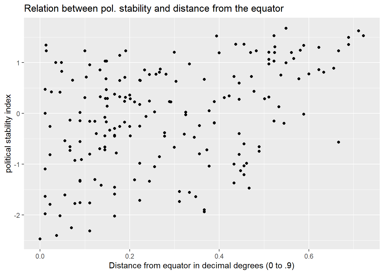
7.2.7 Question 7
What is the correlation coefficient of political stability and latitude? Is it statistically significant?
cor.test(y = world.data$wbgi_pse,
         x = world.data$lp_lat_abst) # correlation and significance
    Pearson's product-moment correlation

data:  x and y
t = 5.8247, df = 185, p-value = 2.492e-08
alternative hypothesis: true correlation is not equal to 0
95 percent confidence interval:
 0.2651437 0.5084328
sample estimates:
      cor
0.3936597
The correlation coefficient ranges from -1 to 1 and is a measure of linear association of two continuous variables. The variables are positively related. That means, as we move away from the equator, we tend to observe higher levels of political stability. This relationship appears to be highly statistically significant.
7.2.8 Question 8
If we move away from the equator, how does political stability change?
A: Political stability tends to increase as we move away from the equator.
7.2.9 Question 9
Does it matter whether we go north or south from the equator?
A: It does not matter whether we go north or south. Our latitude is measured in decimal degrees. Thus, a value of 0.9 could correspond to either the North Pole or the South Pole.