Chapter 1 Introduction to R

1.1 Seminar

Welcome to POL269! Throughout this module, you will not only be learning how to understand the theory and application of quantitative research, but also how to carry it out yourselves. We will be teaching you how to analyse data in R.

In this seminar session, we introduce working with R. We illustrate some basic functionality and help you familiarise yourself with the look and feel of RStudio.

1.1.1 Getting Started

You should by now have received an email instructing you how to set up an RStudio Cloud account and how to access the POL269 section. Enter the project titled Seminar 1.

1.1.2 RStudio

Let’s get acquainted with R. When you start RStudio for the first time, you’ll see three panes:

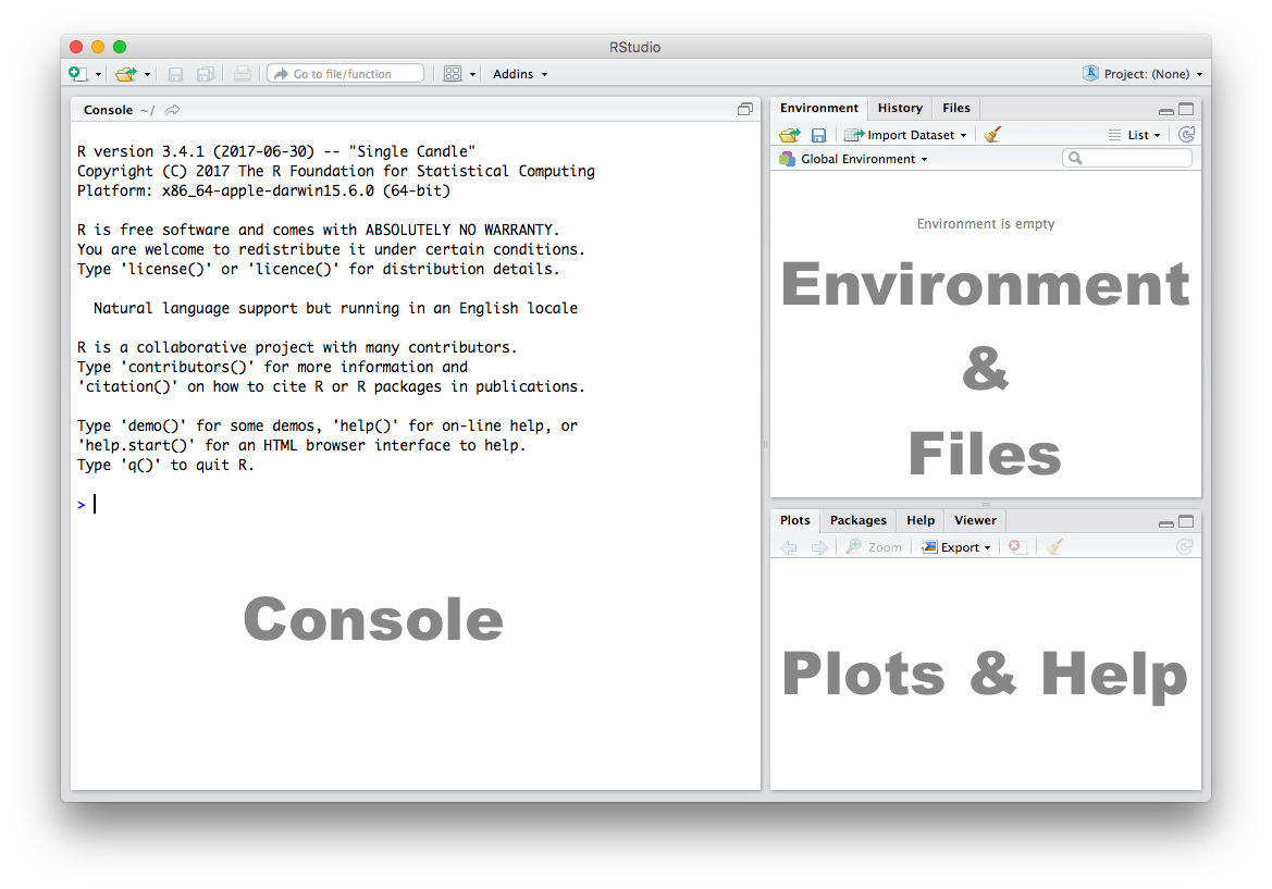
1.1.3 Console

The Console in RStudio is the simplest way to interact with R. You can type some code in the Console and when you press ENTER, R will run that code and give you something back. Depending on what you type, you may see some output in the Console, or if you make a mistake, you may get a warning or an error message. Warnings simply tell you something might have gone wrong, but do not prevent you from getting an output. Errors stop your code in its tracks and tell you something is wrong, so you do not get any output.

Let’s familiarize ourselves with the console by using R as a simple calculator:

2 + 4

[1] 6

2 + 4 is so simple that you could type it into Google and get an answer. But here it is a very basic line of code. The + operator has a meaning in R, and it also understands and reads numbers as they are. So 2 + 4 here is a command, written in R code, and the output of that code is 6. Now that we know how to use the + sign for addition, let’s try some other mathematical operations such as subtraction (-), multiplication (*), and division (/).

10 - 4

[1] 6

5 * 3

[1] 15

7 / 2

[1] 3.5

You can use the cursor or arrow keys on your keyboard to edit your code at the console:
- Use the UP and DOWN keys to re-run something without typing it again
- Use the LEFT and RIGHT keys to edit

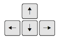Take a few minutes to play around in the console and try different things out. Don’t worry if you make a mistake, you can’t break anything (at least not easily!).

1.1.4 Functions

If all we ever did was write out simple commands like this, R would become very repetitive and time-consuming. Instead, we use functions: a set of instructions that carry out a specific task. Functions, generally, take some input and generate some output. For example, instead of using the + operator for addition, we can use the sum function to add two or more numbers.

sum(1, 4, 10)

[1] 15

In the example above, 1, 4, 10 are the inputs and 15 is the output. A function always requires the use of parenthesis or round brackets (). Inputs to the function are called arguments and go inside the brackets. The output of a function is displayed on the screen but we can also have the option of saving the result of the output. More on this later.

1.1.5 Getting Help

A useful function in R is help, which we can use to display online documentation about a function. For example, if we wanted to know how to use the sum function, we could type help(sum) and look at the online documentation.

help(sum)

The question mark ? can also be used as a shortcut to access online help.

?sum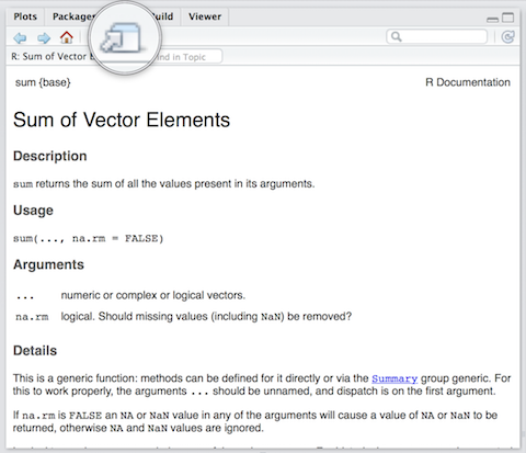

Use the toolbar button shown in the picture above to expand and display the help in a new window.

Help pages for functions in R follow a consistent layout generally including these sections:

Description	A brief description of the function
Usage	The complete syntax or grammar including all arguments (inputs)
Arguments	Explanation of each argument
Details	Any relevant details about the function and its arguments
Value	The output value of the function
Examples	Example of how to use the function

1.1.6 The Assignment Operator

Now we know how to provide inputs to a function using parenthesis or round brackets (), but what about the output of a function?

We use the assignment operator <- for creating or updating objects. If we wanted to save the result of adding sum(1, 4, 10), we would do the following:

myresult <- sum(1, 4, 10)

The line above creates a new object called myresult in our environment and saves the result of the sum(1, 4, 10) in it. To see what’s in myresult, just type it in the console:

myresult

[1] 15

Take a look at the Environment pane in RStudio and you’ll see myresult there.

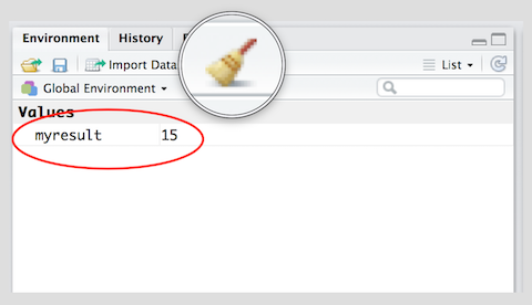
To delete all objects from the environment, you can use the broom button as shown in the picture above.

We called our object myresult but we can call it anything as long as we follow a few simple rules. Object names can contain upper or lower case letters (A-Z, a-z), numbers (0-9), underscores (_) or a dot (.) but all object names must start with a letter. Choose names that are descriptive and easy to type.

Good Object Names	Bad Object Names
result	a
myresult	x1
my.result	this.name.is.just.too.long
my_result
data1

A good principle to follow is to name your objects so that other people – including, most importantly your future self – can easily work out what they are. Every person who has ever written code has experienced coming back to it later and having to start from scratch because they can’t remember what everything means. Try to avoid this, if possible, by getting into good habits now!

1.1.7 Scripts

The Console is great for simple tasks but if you’re working on a project you should save your work in some sort of a document or a file. Scripts in R are just plain text files that contain R code. You can edit a script just like you would edit a file in any word processing or note-taking application. You can also run code directly from it, but that code doesn’t disappear afterwards. This makes it easy to edit and improve your code over time, and makes your work transparent.

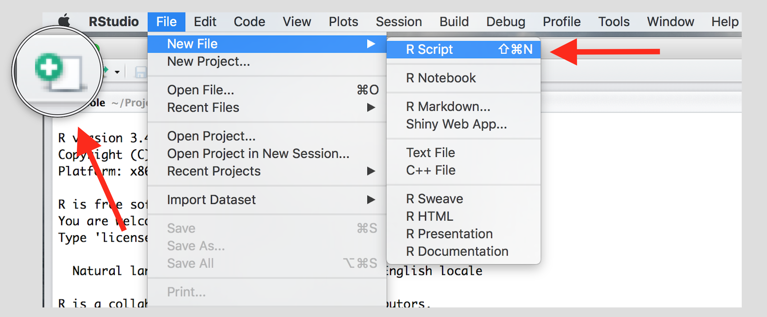
Create a new script using the menu or the toolbar button as shown below.

Once you’ve created a script, it is generally a good idea to give it a meaningful name and save it immediately. For our first session save your script as seminar1.R

Familiarize yourself with the script window in RStudio, and especially the two buttons labeled Run and Source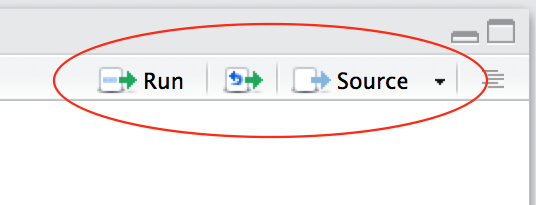

There are a few different ways to run your code from a script.

One line at a time	Place the cursor on the line you want to run and hit CTRL-ENTER or use the Run button
Multiple lines	Select the lines you want to run and hit CTRL-ENTER or use the Run button
Entire script	Use the Source button

1.1.8 Working with Data

So we know that the basic premise of R is that we run code, mostly functions, on objects. What can we do with this? In most cases of quantitative research or data science, we use this process to manipulate and analyse quantitative data. In R, we typically deal with dataframes. These are like spreadsheets of data that you know from Microsoft Excel, arranged in columns and rows. But ‘data’, in general, just means information that is gathered together in some way.

It is easy to create our own dataframe, using the data.frame() function, then see what we have created:

# create some data
my_data <- data.frame(0:10, # first column is numbers from 0 to 10
                      20:30) # second column is numbers from 20 to 30

# summarise dataframe in the console
my_data

   X0.10 X20.30
1      0     20
2      1     21
3      2     22
4      3     23
5      4     24
6      5     25
7      6     26
8      7     27
9      8     28
10     9     29
11    10     30

You can run this code line by line, or all in one go, as you please. Just make sure you write it in the script and run it from there, as explained above. There are a few things here you haven’t seen before. First, everything after a # (known as a comment) is ignored. Second, the colon : tells R to create a sequence of all the numbers in the range specified. We will talk more about sequences next week.

Looking at my_data you’ll see that the columns have strange titles. We can overwrite this using colnames().

# add/change column names
colnames(my_data) <- c("tens", "twenties")

# did it work?
my_data

   tens twenties
1     0       20
2     1       21
3     2       22
4     3       23
5     4       24
6     5       25
7     6       26
8     7       27
9     8       28
10    9       29
11   10       30

There is another new function introduced here: c(). This stands for concatenate which basically means ‘bring together’. It is what we use in R to create vectors. We will discuss this more next week.

This dataframe shows you, at a basic level, the format we use to deal with data in R, but it is not very interesting. Usually, we take data from external sources such as surveys or official statistics, import them into R, and analyse this more interesting data. In later seminars we will use datasets on topics such as election results, COVID-19 and political systems. Today we use a very small dataset of the heights and weights of some women in the USA.

This dataset is available by default in R, so we can simply load it using the data function. You can see a full list of the data stored by default in R by running data() (with no arguments in the brackets). Usually we will need to use different functions, such as read.csv, to load more interesting, comprehensive datasets from the internet. We will do this in future tutorials.

# open the default 'women' dataset from within R
data(women)

We can confirm the type of object ‘women’ is using class():

class(women)

[1] "data.frame"

We can also look at the contents of the object. Data frames can sometimes be too large to show in the console, so we usually look at the beginning of the dataset - head() - or the end - tail().

# show first six rows
head(women)

  height weight
1     58    115
2     59    117
3     60    120
4     61    123
5     62    126
6     63    129

# show last six rows
tail(women)

   height weight
10     67    142
11     68    146
12     69    150
13     70    154
14     71    159
15     72    164

Just looking at the numbers like this, it is not easy to see how they are related. A useful way to understand any relationship between different variables is to plot them. It is easy to generate plots in R. We’ll explore this a lot more in future tutorials.

# scatterplot
plot(women$height, women$weight)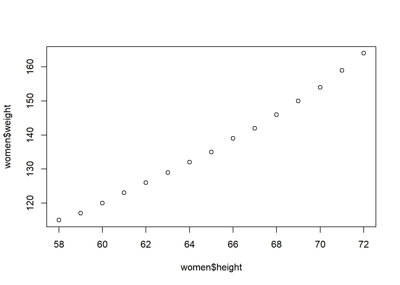

To get to know a bit more about the file you have loaded R has a number of useful functions. We can use these to find out how many columns (variables) and rows (cases) the dataframe (dataset) contains.

# number of columns
ncol(women)

[1] 2

# number of rows
nrow(women)

[1] 15

# column headings
names(women)

[1] "height" "weight"

# or
colnames(women)

[1] "height" "weight"

Sometimes we are only interested in certain parts of dataframes. In R there are two ways of selecting an individual column. The first uses the $ symbol to select columns.

# select the weight column

women_weight <- women$weight

head(women_weight)

[1] 115 117 120 123 126 129

A second approach is to use [Row, Column]:

# select only second column
women_weight <- women[,2] # leave the row section blank to get all rows

head(women_weight)

[1] 115 117 120 123 126 129

This same approach can be used to select certain rows:

# select only first row
one_woman <- women[1,] # leave the column section blank to get all column

one_woman

  height weight
1     58    115

# get only the first woman's weight
one_weight <- women[1,1]

one_weight

[1] 58

This seminar has introduced you to the basics of using R. From next week onwards, we will begin to apply this more practically to analysing and learning about our data. To make sure you have grasped the basics and are thinking about R in the right way, try out the exercises below before next time.

1.1.9 Exercises

Create a script and call it assignment01. Save your script.
Download this cheat-sheet and go over it. You won’t understand most of it right away. But it will become a useful resource. Look at it often.
Calculate the square root of 1369 using the sqrt() function.
Square the number 13 using the ^ operator.
What is the result of summing all numbers from 1 to 10?
Load up the default data quakes from R in the same way you loaded the women data. Use ?quakes to find out more about this dataset.

Look at the first 6 rows of quakes.
Using the [Row, Column] approach, find out how many stations reported the 18th earthquake in the dataset.
Extract the mag column from the quakes dataset using the $ operator. Call this new object quake_mags.
Generate a simple plot of the number of stations reporting an earthquake (stations) by its magnitude (mag). What do you notice about the relationship? Why might this be the case?

Save your R script by pressing the Save button in the script window.