3.2 Solutions
- Load this dataset about penguins:
# read in the penguins datafile

penguins <- readRDS(url("https://github.com/QMUL-SPIR/Public_files/blob/master/datasets/penguins.rds?raw=true"))- Inspect the dataframe using
head(),names(), anddim(). - Create a histogram of penguin flipper length.
- How does the distribution of flipper length vary by species? Take your histogram and add a
facet_wraplayer to see this. - Add a title to the faceted plot using the
ggtitle()layer. If you need help, try?ggtitle. - Create a scatterplot to show the relationship between bill depth and bill length. How would you describe this relationship?
- How does this relationship change when we break it down into species? Rewrite your scatterplot code so that the colour of the points varies by species.
- Save this plot using
ggsave(). - What do you observe? Describe your findings.
3.2.1 Exercise 1
Load this dataset about penguins:
# read in the penguins datafile

penguins <- readRDS(url("https://github.com/QMUL-SPIR/Public_files/blob/master/datasets/penguins.rds?raw=true"))
3.2.2 Exercise 2
- Inspect the dataframe using
head(),names(), anddim().
head(penguins)# A tibble: 6 x 8
species island bill_length_mm bill_depth_mm flipper_length_~ body_mass_g sex
<fct> <fct> <dbl> <dbl> <int> <int> <fct>
1 Adelie Torge~ 39.1 18.7 181 3750 male
2 Adelie Torge~ 39.5 17.4 186 3800 fema~
3 Adelie Torge~ 40.3 18 195 3250 fema~
4 Adelie Torge~ NA NA NA NA <NA>
5 Adelie Torge~ 36.7 19.3 193 3450 fema~
6 Adelie Torge~ 39.3 20.6 190 3650 male
# ... with 1 more variable: year <int>names(penguins)[1] "species" "island" "bill_length_mm"
[4] "bill_depth_mm" "flipper_length_mm" "body_mass_g"
[7] "sex" "year" dim(penguins)[1] 344 83.2.3 Exercise 3
Create a histogram of penguin flipper length.
library(ggplot2)

flipper_hist <- ggplot(penguins, aes(x = flipper_length_mm)) +
  geom_histogram()

flipper_hist
`stat_bin()` using `bins = 30`. Pick better value with `binwidth`.Warning: Removed 2 rows containing non-finite values (stat_bin).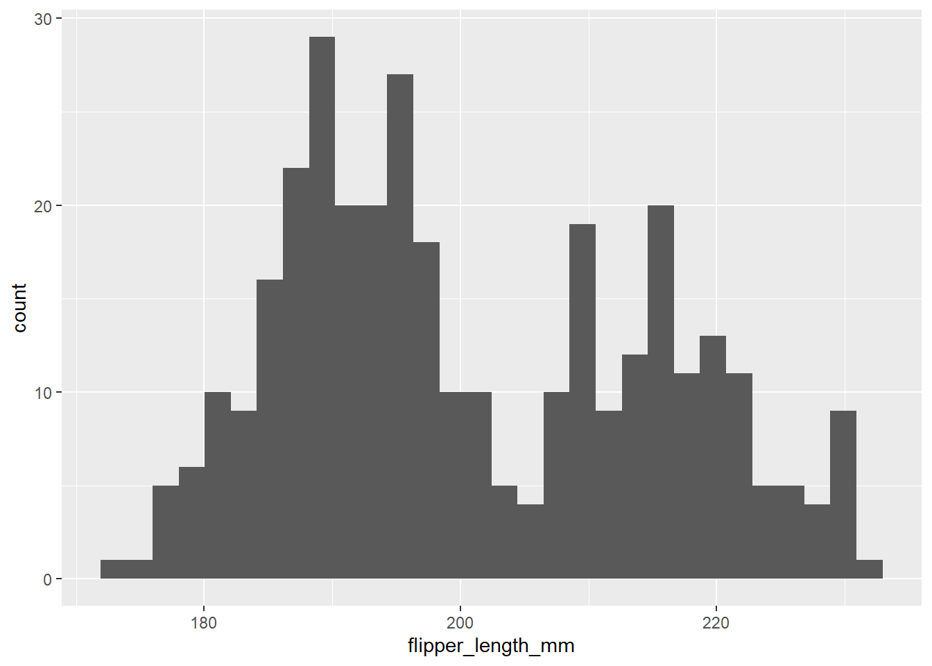
3.2.4 Exercise 4
How does the distribution of flipper length vary by species? Take your histogram and add a facet_wrap layer to see this.
flipper_hist + facet_wrap(~ species)`stat_bin()` using `bins = 30`. Pick better value with `binwidth`.Warning: Removed 2 rows containing non-finite values (stat_bin).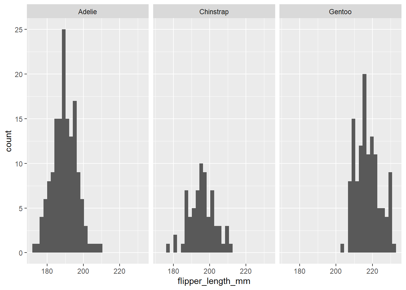
3.2.5 Exercise 5
Add a title to the faceted plot using the ggtitle() layer. If you need help, try ?ggtitle.
flipper_hist +
  facet_wrap(~ species) +
  ggtitle("Flipper lengths of different species of penguin")
`stat_bin()` using `bins = 30`. Pick better value with `binwidth`.Warning: Removed 2 rows containing non-finite values (stat_bin).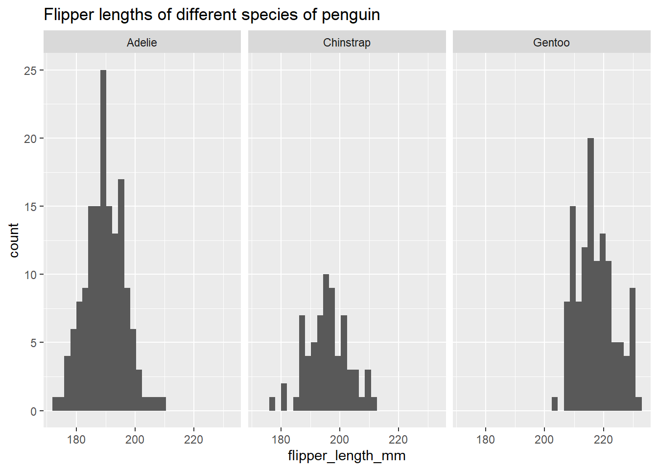
3.2.6 Exercise 6
Create a scatterplot to show the relationship between bill depth and bill length. How would you describe this relationship?
bill_scatter <- ggplot(penguins, aes(x = bill_depth_mm, y = bill_length_mm)) +
  geom_point()

# hint: adding a layer of geom_smooth(method = "lm")
# will help you work out whether the relationship is positive or negative

bill_scatter
Warning: Removed 2 rows containing missing values (geom_point).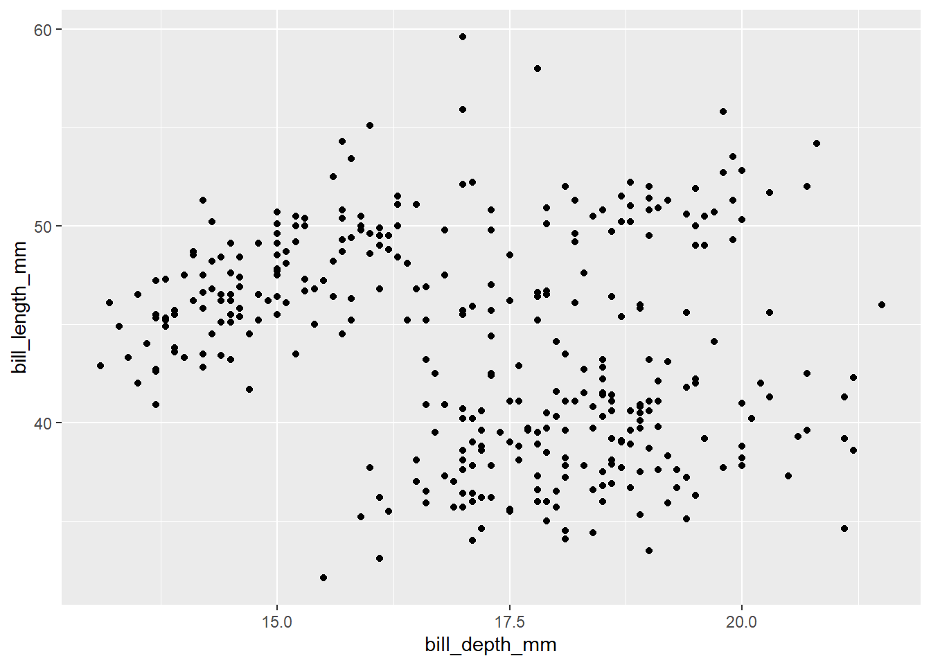
There appears to be a weak negative relationship between bill depth and bill length – deeper bills tend to be shorter in length.
3.2.7 Exercise 7
How does this relationship change when we break it down into species? Rewrite your scatterplot code so that the colour of the points varies by species.
bill_scatter_species <- ggplot(penguins, aes(x = bill_depth_mm, y = bill_length_mm)) +
  geom_point(aes(colour = species))

bill_scatter_species
Warning: Removed 2 rows containing missing values (geom_point).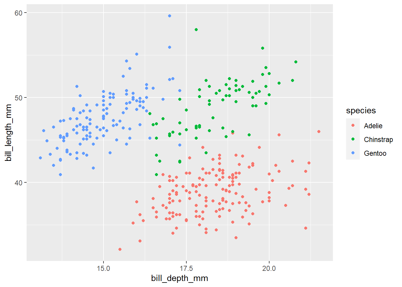
3.2.8 Exercise 8
Save this plot using ggsave().
ggsave("bill_scatter_species.pdf", scale = 2)Saving 14 x 10 in imageWarning: Removed 2 rows containing missing values (geom_point).3.2.9 Exercise 9
Now, we can see that, within each species of penguin, there is a positive relationship between bill depth and length. This relationship is masked by the fact that different species of penguin have different sized bills overall. What we have uncovered here, through data visualisation, is an example of Simpson’s paradox.