Chapter 6 T-test for Difference in Means and Hypothesis Testing

library(tidyverse)

6.1 Seminar

We’ll be using data on constituency-level results of the 2016 referendum on membership of the EU. Load in the data and familiarise yourself with the codebook below.

# load in brexit data
brexit <- readRDS(url('https://github.com/QMUL-SPIR/Public_files/blob/master/datasets/BrexitResults.rds?raw=true'))

Warning in readRDS(url("https://github.com/QMUL-SPIR/Public_files/blob/master/
datasets/BrexitResults.rds?raw=true")): strings not representable in native
encoding will be translated to UTF-8

Warning in readRDS(url("https://github.com/QMUL-SPIR/Public_files/blob/master/
datasets/BrexitResults.rds?raw=true")): input string 'Ynys Môn' cannot be
translated to UTF-8, is it valid in 'UTF-8' ?

Variable	Description
`pano`	Press Association constituency number.
`ConstituencyName`	Name of the Constituency according to the Electoral Commission.
`BrexitVote`	Estimated share of votes for Brexit in the EU referendum in each constituency (Hanretty, 2017).
`London`	0 if the constituency is located outside of London and 1 if it is inside. It’s a factor variable.
`Country`	Scotland, England or Wales.
`Region`	Regional divisions of Great Britain.
`Winner15`	Party that won in the constituency in 2015.
`Con15`	Share of votes for the Conservatives in 2015.
`Lab15`	Share of votes for Labour in 2015.
`LD15`	Share of votes for the Liberal Democrats in 2015.
`SNP15`	Share of votes for the Scottish National Party in 2015.
`PC15`	Share of votes for Plaid Cymru in 2015.
`UKIP15`	Share of votes for UKIP in 2015.
`Green15`	Share of votes for the Greens in 2015.
`Other15`	Share of votes for other parties in 2015.
`Majority15`	Difference between the winner and the second party in each constituency.
`Turnout15`	Turnout in each constituency in 2015.
`BornUK`	% of people in the constituency born in the UK (Census 2011).
`PercFemale`	% of women in the constituency (Census 2011).
`PopulationDensity`	Average number of people per square mile in each constituency (Census 2011).

We can get summary statistics of each variable in the dataset by using the summary() function over the dataset.

summary(brexit)

      pano       ConstituencyName     BrexitVote              London   
 Min.   :  1.0   Length:632         Min.   :20.54   Out of London:559  
 1st Qu.:165.8   Class :character   1st Qu.:45.39   London       : 73  
 Median :327.5   Mode  :character   Median :53.74                      
 Mean   :327.5                      Mean   :52.07                      
 3rd Qu.:488.2                      3rd Qu.:60.14                      
 Max.   :650.0                      Max.   :74.96                      
                                                                       
     Country                Region                       Winner15  
 England :533   South East     : 84   Conservative           :330  
 Scotland: 59   North West     : 75   Labour                 :232  
 Wales   : 40   London         : 73   Scottish National Party: 56  
                West Midlands  : 59   Liberal Democrat       :  8  
                Scotland       : 59   Plaid Cymru            :  3  
                East of England: 58   (Other)                :  2  
                (Other)        :224   NA's                   :  1  
     Con15            Lab15             LD15             SNP15      
 Min.   : 4.673   Min.   : 4.506   Min.   : 0.7497   Min.   :33.79  
 1st Qu.:22.174   1st Qu.:17.700   1st Qu.: 2.9757   1st Qu.:44.93  
 Median :41.021   Median :31.280   Median : 4.5944   Median :50.94  
 Mean   :36.662   Mean   :32.350   Mean   : 7.8217   Mean   :50.16  
 3rd Qu.:50.845   3rd Qu.:44.389   3rd Qu.: 8.5784   3rd Qu.:55.64  
 Max.   :65.876   Max.   :81.301   Max.   :51.4909   Max.   :61.91  
 NA's   :1        NA's   :1        NA's   :1         NA's   :573    
      PC15            UKIP15          Green15           Other15       
 Min.   : 3.506   Min.   : 1.033   Min.   : 0.8982   Min.   : 0.1179  
 1st Qu.: 5.686   1st Qu.: 9.807   1st Qu.: 2.6407   1st Qu.: 0.4416  
 Median : 9.780   Median :13.923   Median : 3.6148   Median : 0.7820  
 Mean   :12.792   Mean   :13.488   Mean   : 4.1832   Mean   : 1.5540  
 3rd Qu.:14.099   3rd Qu.:17.284   3rd Qu.: 4.7401   3rd Qu.: 1.3355  
 Max.   :43.932   Max.   :44.432   Max.   :41.8300   Max.   :64.4733  
 NA's   :592      NA's   :18       NA's   :64        NA's   :253      
   Majority15         Turnout15         BornUK        PercFemale   
 Min.   : 0.06315   Min.   :51.26   Min.   :40.73   Min.   :46.95  
 1st Qu.:12.85206   1st Qu.:63.00   1st Qu.:86.42   1st Qu.:50.57  
 Median :24.35840   Median :67.09   Median :92.48   Median :50.98  
 Mean   :24.25556   Mean   :66.38   Mean   :88.15   Mean   :50.93  
 3rd Qu.:34.58712   3rd Qu.:70.33   3rd Qu.:95.42   3rd Qu.:51.39  
 Max.   :72.33029   Max.   :81.94   Max.   :98.02   Max.   :53.14  
                                                                   
 PopulationDensity  
 Min.   :  0.05572  
 1st Qu.:  2.63869  
 Median :  9.59660  
 Mean   : 20.22218  
 3rd Qu.: 31.29706  
 Max.   :146.38461

6.1.1 T-test (one sample hypothesis test)

A knowledgeable friend tells you that the average population of women in British constituencies is 52%. You would like to know whether she is right. To that end, you assume that her claim is the population mean. Unfortunately, you don’t have access to the data we have here, so you go and collect your own data, on 400 randomly sampled Britsh constituencies.

brexit_400 <- sample_n(brexit, 400)

You then estimate the mean of PercFemale in your sample. If the difference is large enough, so that it is unlikely that it could have occurred by chance alone, you can probably reject your friend’s claim.

So, first you take the mean of the PercFemale variable. Bear in mind, your answer will be slightly different.

mean(brexit_400$PercFemale)

[1] 50.94187

Your friend’s claim is quite close. Substantively, the difference between your friend’s claim and your estimate is small, but you could still find that the difference is statistically significant (i.e. that it’s a noticeable systematic difference).

Because we do not have information on all constituencies, your 50.94 is an estimate and the true population mean – the population here would be all constituencies – may be 52% as your friend claims. You can test this statistically.

In statistics jargon: you would like to test whether your estimate is statistically different from the 52% figure (the null hypothesis) suggested by your friend. Put differently, you would like to know the probability that you estimate 50.94 if the true mean of all constituencies is 52%.

Recall that the standard error of the mean (which is the estimate of the true standard deviation of the population mean) is estimated as:

\[ \frac{s_{Y}}{\sqrt{n}} \]

Before you estimate the standard error, you need to get $n$ (the number of observations). You can save the number of observations in an object that you call n.

n <- length(brexit_400$PercFemale)
n

[1] 400

With the function length(brexit_400$PercFemale) you get all observations in the data. Now, take the standard error of the mean.

# standard error calculation
se.y_bar <- sd(brexit_400$PercFemale) / sqrt(n)

We know that 1 standard error is one average deviation from the population mean. The sampling distribution is approximately normal. 95 percent of the observations under the normal distribution are within 2 (1.96, to be precise) standard deviations of the mean.

You can construct the confidence interval within which the population mean lies with 95 percent probability in the following way. First, take the mean of PercFemale. That’s the sample mean and not the population mean. Second, go 1.96 standard errors to the left of it. This is the lower bound of the confidence interval. Third, go 1.96 standard deviations to the right of the sample mean. That is the upper bound of the confidence interval.

The 95 percent confidence interval around the sample means gives the interval within which the population mean lies with 95 percent probability.

You want to know what the population mean is, so you want the confidence interval to be as narrow as possible. The narrower the confidence interval, the more precise your estimate of the population mean. For instance, saying the population mean of is between 48% and 52% is more precise than saying the population mean is between 45% and 55%. Both would give the same mean estimate of 50%, though.

You construct the confidence interval with the standard error. That means, the smaller the standard error, the more precise the estimate. The formula for the 95 percent confidence interval is:

\[ \bar{Y} \pm 1.96 \times SE(\bar{Y}) \]

You can now construct your confidence interval. Your sample is large enough to assume that the sampling distribution is approximately normal. So, go $1.96$ standard deviations to the left and to the right of the mean to construct your $95\%$ confidence interval. Remember that your results will be slightly different.

# lower bound
lb <- mean(brexit_400$PercFemale) - 1.96 * se.y_bar
# upper bound
ub <- mean(brexit_400$PercFemale) + 1.96 * se.y_bar
# results (the population mean lies within this interval with 95% probability)
lb # lower bound

[1] 50.86063

mean(brexit_400$PercFemale) # sample mean

[1] 50.94187

ub # upper bound

[1] 51.0231

You can make this look a little more like a table like so:

ci <- cbind(lower_bound = lb, 
            mean = mean(brexit_400$PercFemale), 
            upper_bound = ub)
ci

     lower_bound     mean upper_bound
[1,]    50.86063 50.94187     51.0231

The cbind() function stands for column-bind and creates a $1\times3$ matrix.

So you are $95\%$ confident that the average proportion of females in UK constituencies is between 50.86% and 51.02% . You can see that you are quite certain about your estimate and can be quite confident in rejecting your friend’s claim.

A different way of describing our finding is to emphasize the logic of (hypothetical) repeated sampling. In a process of repeated sampling you can expect that the confidence interval that we calculate for each sample will include the true population value $95\%$ of the time.

6.1.1.1 The t value

You can now estimate the t value. Recall that your friend claimed that the population mean was 53%. This is the null hypothesis that you wish to falsify. You estimated something else in your data, namely 50.9418664. The t value is the difference between your estimate (the result you got by looking at data) and the population mean under the null hypothesis, divided by the standard error of the mean.

\[ \frac{ \bar{Y} - \mu_0 } {SE(\bar{Y})} \]

Where $\bar{Y}$ is the mean in your data, $\mu_0$ is the population mean under the null hypothesis and $SE(\bar{Y})$ is the standard error of the mean.

Let’s compute this. Your results will be slightly different.

t.value <- (mean(brexit_400$PercFemale) - 52) / se.y_bar

t.value

[1] -25.52963

Look at the formula until you understand what is going on. In the numerator you take the difference between your estimate and the population mean under the null hypothesis. In expectation that difference should be 0 — assuming that the null hypothesis is true. The larger that difference, the less likely it is that the null hypothesis is true.

Dividing by the standard error transforms the units of the difference into standard deviations. Before transforming the units, the difference was in the units of the variable itself. By dividing by the standard error, you have normalised the variable. Its units are now standard deviations from the mean.

Assume that the null hypothesis is true. In expectation the difference between your estimate in the data and the population mean should be 0 standard deviations. The more standard deviations your estimate is away from the population mean under the null hypothesis, the less likely it is that the null hypothesis is true.

Within 1.96 standard deviations from the mean lie 95 percent of all observations. That means, it is very unlikely that the null hypothesis is true, if the difference that we estimated is further than 1.96 standard deviations from the mean. How unlikely? For this, you would need the p value, for the exact probability. However, the probability is less than 5 percent if the estimated difference is more than 1.96 standard deviations from the population mean under the null hypothesis.

Back to the t value. We estimated a t value of -25.5296327. That means that a sample estimate of 50.9418664 is -25.5296327 standard deviations from the population mean under the null hypothesis — which is 53%.

This t value suggests that your sample estimate would be -25.5296327 standard deviations away from the population mean under the null. That is very unlikely. You can very confidently reject the null hypothesis in this case. Your friend is very unlikely to be right, based on your findings.

6.1.1.2 The p value

Let’s estimate the precise p-value by calculating how likely it would be to observe a t-statistic of -25.5296327 from a t-distribution with n - 1 (399) degrees of freedom.

The function pt() can be used to get the p-value associated with a given t score. However, t-scores can be negative, which confuses the calculation. Because we are dealing with symmetric, two-tailed distributions, we can account for this by just taking the absolute value using abs(). This removes the negative sign. Then, we set lower.tail = FALSE to get the probability to the right – that is, of all values above – of our t value. We then multiply this by two to get our two-tailed p value. That is, we get the probability that we see a t.value in the right tail or in the left tail of the distribution.

# calculate p value
p.value <- 2* pt(abs(t.value), df = (n-1), lower.tail = FALSE)

p.value

[1] 6.429686e-86

Our p-value is so small that R isn’t even displaying it as a decimal number, but using scientific notation instead, the shorten the output. This number is very close to zero. It is extremely unlikely that our sample would give us the estimated mean that it gave us if the true population mean were 52%, as your friend said.

Let’s verify our result using the the t-test function t.test(). The syntax of the function is:

t.test(formula, mu, alt, conf.level)

Lets have a look at the arguments.

Arguments	Description
`formula`	Here, we input the vector that we calculate the mean of. For the one-sample t test, in our example, this is the mean of `PercFemale`. Below we talk about two-sample tests.
`mu`	Here, we set the null hypothesis. The null hypothesis is that the true population mean is 52%. Thus, we set `mu = 52`.
`alt`	There are two alternatives to the null hypothesis that the difference in means is zero. The difference could either be smaller or it could be larger than zero. To test against both alternatives, we set `alt = "two.sided"`.
`conf.level`	Here, we set the level of confidence that we want in rejecting the null hypothesis. Common confidence intervals are: 95% (0.95), 99% (0.99), and 99.9% (0.999)—they correspond to alpha levels of 0.05, 0.01 and 0.001 respectively.

t.test(brexit_400$PercFemale, 
       mu = 52, 
       alt = "two.sided",
       conf.level = 0.95)


    One Sample t-test

data:  brexit_400$PercFemale
t = -25.53, df = 399, p-value < 2.2e-16
alternative hypothesis: true mean is not equal to 52
95 percent confidence interval:
 50.86038 51.02335
sample estimates:
mean of x 
 50.94187

The results are similar. This p value might look quite different, but that’s because 2.2e-16 is the smallest value R’s statistical calculations provide. Beyond this, it is of no use to us to know how small a number is, because this number is already so close to 0. We can conclude that you are able to reject the null hypothesis suggested by your friend that the population mean is equal to 52% with considerable confidence.

6.1.1.3 Critical Values

In social sciences, we usually operate with an alpha level of 0.05. That means, we reject the null hypothesis if the p value is smaller than 0.05. Or put differently, we reject the null hypothesis if the 95 percent confidence interval does not include the population mean under the null hypothesis — which is always the case if our estimate is further than two standard errors from the mean under null hypothesis (usually 0).

We said earlier that the critical value is 1.96 for an alpha level of 0.05. That is true in large samples where the distribution of the t value follows a normal distribution. 95 percent of all observations are within 1.96 standard deviations of the mean.

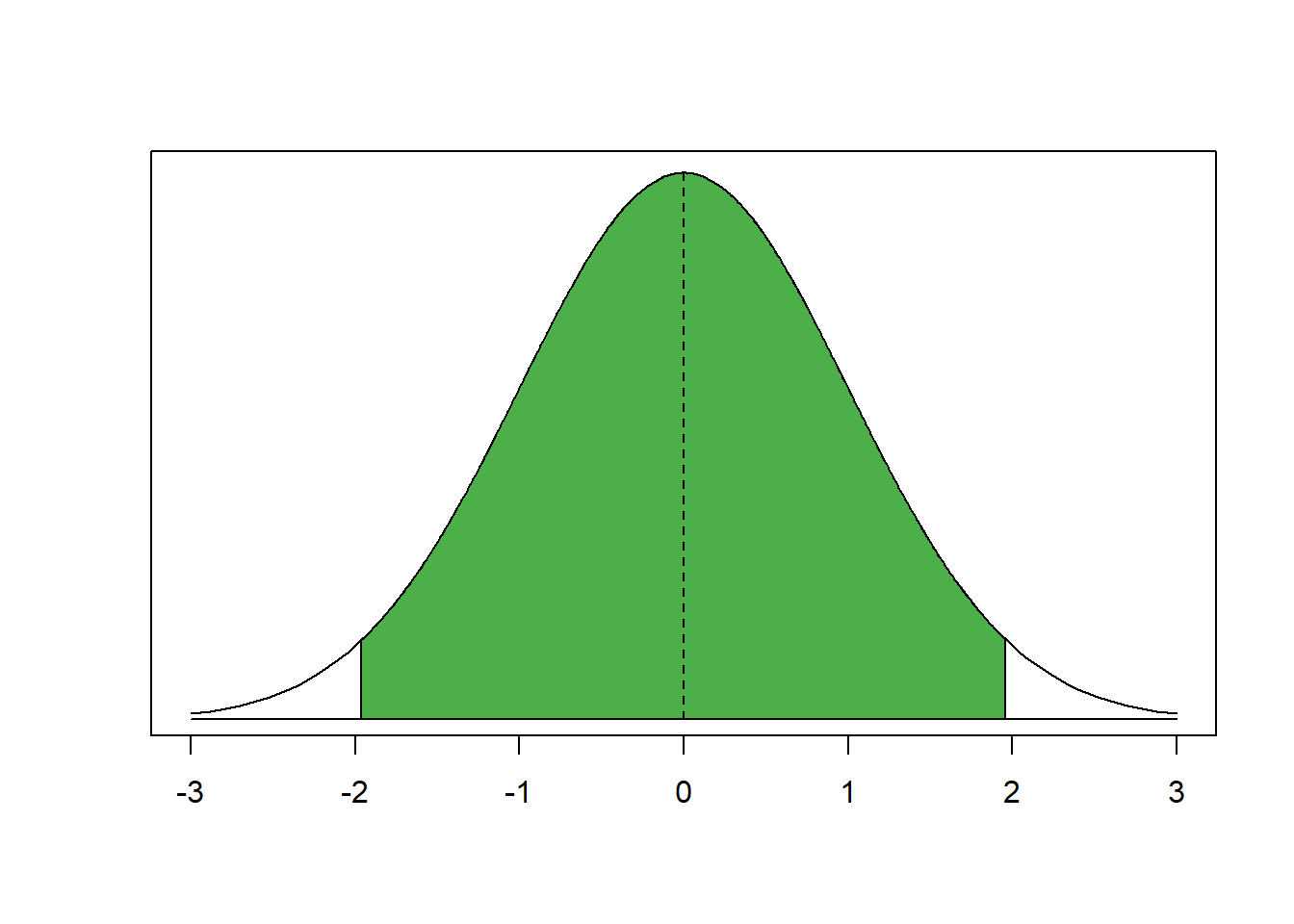
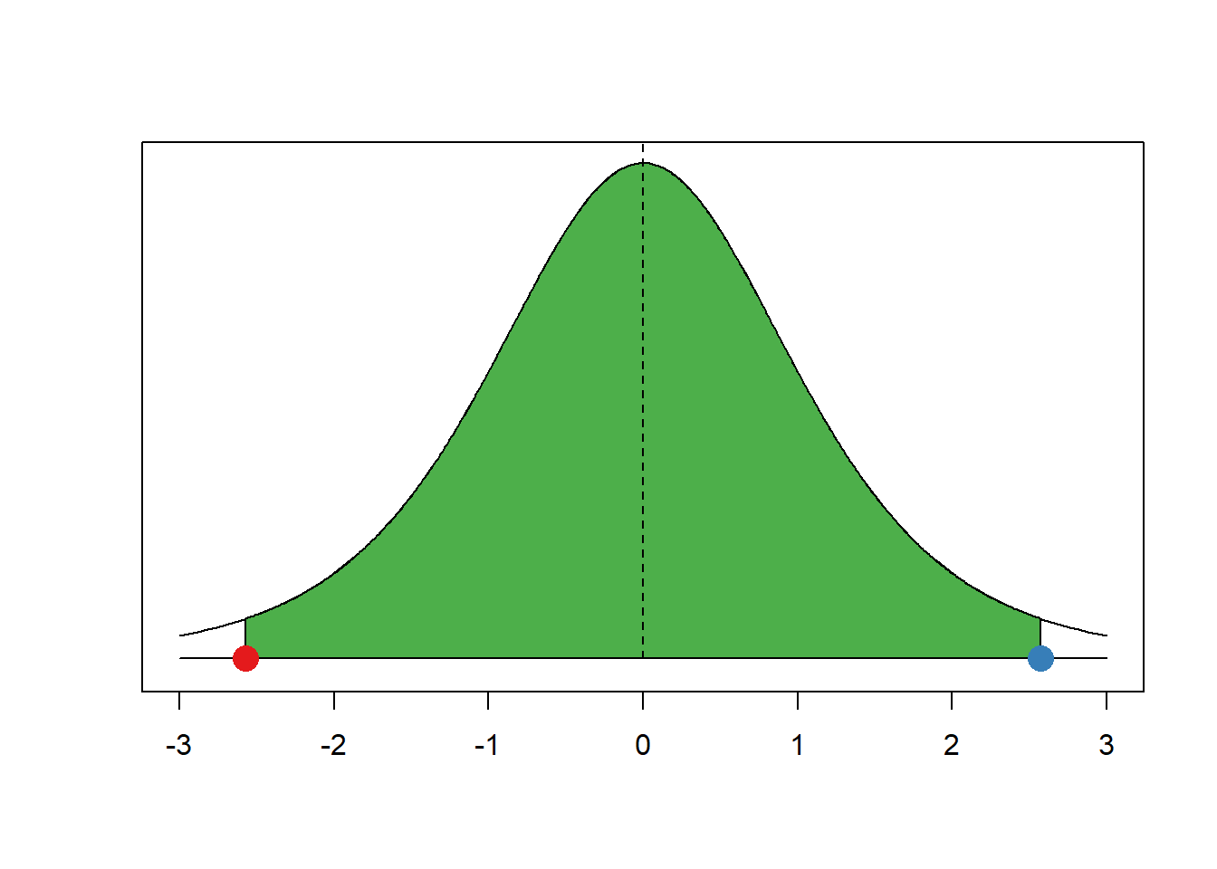
The green area under the curve covers 95 percent of all observations. There are 2.5 percent in each tail. We reject the null hypothesis if our estimate is in the tails of the distribution. It must be further than 1.96 standard deviations from the mean. But how did we know that 95 percent of the area under the curve is within 1.96 standard deviations from the mean?

Separate the curve in your mind into 3 pieces. The left tail covers 2.5 percent of the area under the curve. The green middle bit covers 95 percent and the right tail again 2.5 percent. Now think of these as cumulative probabilities. The left tail ends at 2.5 percent cumulative probability. The green area ends at 97.5 percent cumulative probability and the right tail ends at 100 percent.

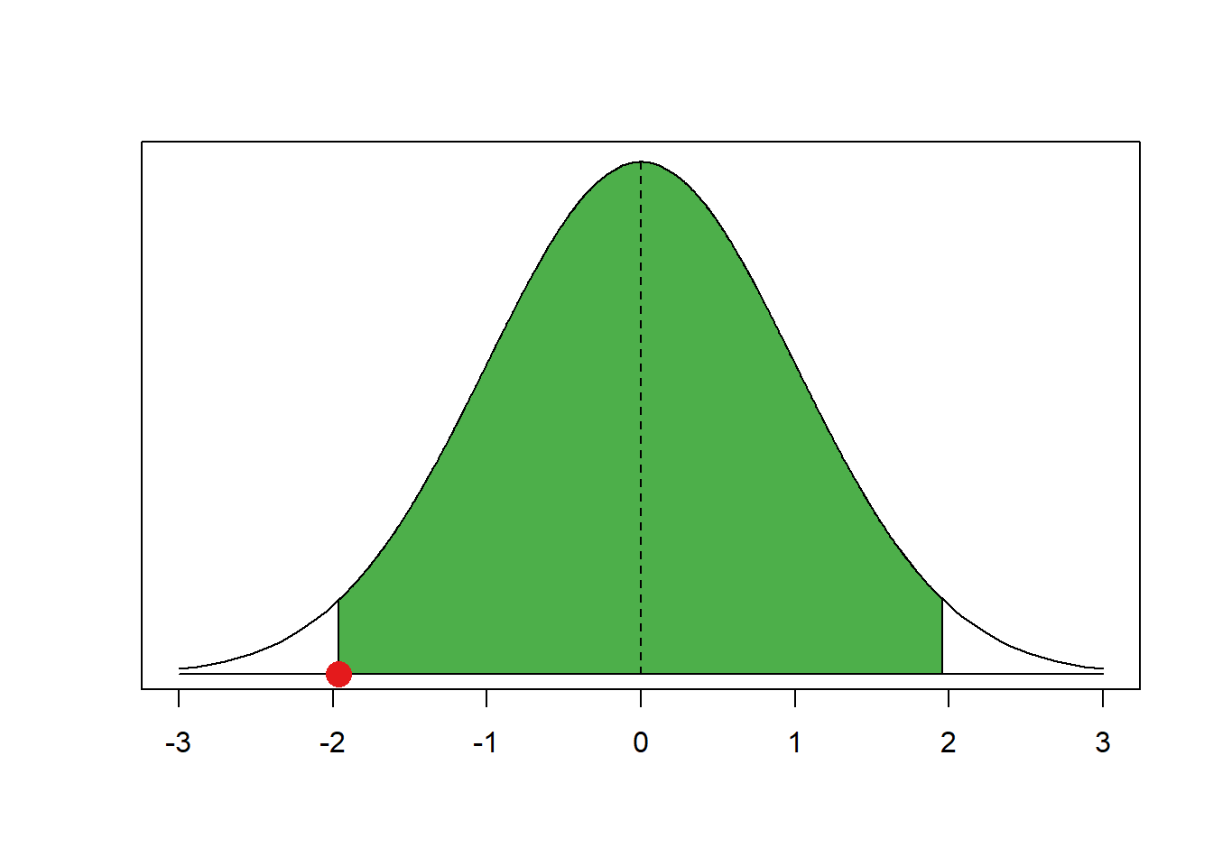
The critical value is were the left tail ends or the right tail starts (looking at the curve from left to right). Let’s get the value where the cumulative probability is 2.5 percent—where the left tail ends.

qnorm(0.025, mean = 0, sd = 1)

[1] -1.959964

If you look at the x-axis of our curve that is indeed where the left tail ends. We add a red dot to our graph to highlight it.

Now, let’s get the critical value of where the right tail starts. That is at the cumulative probability of 97.5 percent.

qnorm(0.975, mean = 0, sd = 1)

[1] 1.959964

As you can see, this is the same number, only positive instead of negative. That’s always the case because the normal distribution is symmetrical. Let’s add that point in blue to our graph.

This is how we get the critical value for the 95 percent confidence interval. Back in the day you would have had to look up critical values in critical values tables at the end of statistics textbooks (you can find the tables in Kellstedt and Whitten, for example).

As you can see our red and blue dots are the borders of the green area, the 95 percent interval around the mean. You can get the critical values for any other interval (e.g., the 99 percent interval) similar to what we did just now.

We now do the same for the t distribution. In the t distribution, the critical value depends on the shape of the t distribution which is characterised by its degrees of freedom. Let’s consider a t distribution with 5 degrees of freedom.

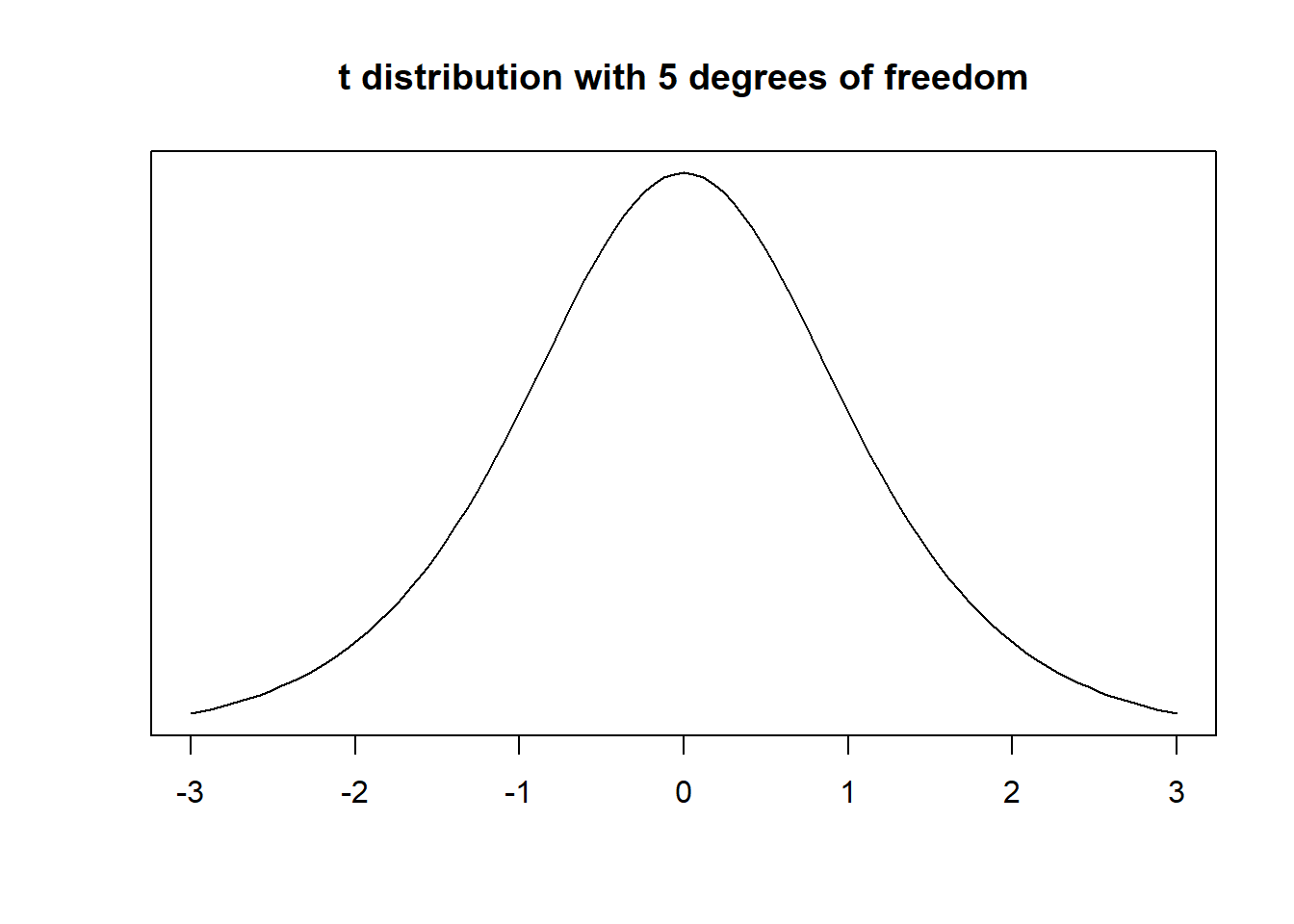
Although, it looks like a standard normal distribution, it is not. The t with 5 degrees of freedom has fatter tails. We show this by overlaying the t with a standard normal distribution.

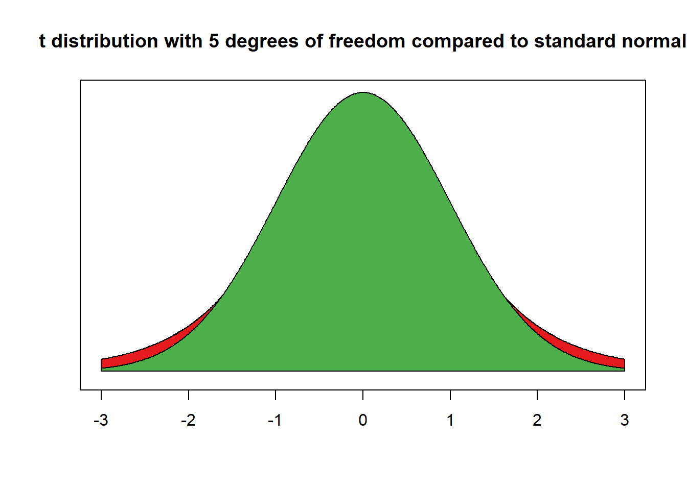
The red area is the difference between the standard normal distribution and the t distribution with 5 degrees of freedom.

The tails are fatter and that means that the probabilities of getting a value somewhere in the tails is larger. Let’s calculate the critical value for a t distribution with 5 degrees of freedom.

# value for cumulative probability 95 percent in the t distribution with 5 degrees of freedom
qt(0.975, df = 5)

[1] 2.570582

See how much larger that value is than 1.96. Under a t distribution with 5 degrees of freedom 95 percent of the observations around the mean are within the interval from negative 2.5705818 to positive 2.5705818.

Let’s illustrate that.

Remember the critical values for the t distribution are always more extreme or similar to the critical values for the standard normal distribution. If the t distribution has few degrees of freedom, the critical values (for the same percentage area around the mean) are much more extreme. If the t distribution has many degrees of freedom, the critical values are very similar.

6.1.2 T-test (difference in means)

Now, working again with our main dataset, we are interested in whether there is a difference in average Brexit vote share between constituencies inside and outside of London. Put more formally, we are interested in the difference between two conditional means. Recall that a conditional mean is the mean in a subpopulation such as the mean of Brexit vote share given that the country is in London (conditional mean 1).

The t-test is the appropriate test statistic. Our interval-level dependent variable is BrexitVote, which is the percentage of people who voted to leave. Let’s look at the distribution of this variable.

brexit_hist <- ggplot(data = brexit, aes(BrexitVote)) +
  geom_histogram() +
  labs(x = "Constituency-level percentage voting leave",
       y = "Frequency",
       title = "Distribution of constituency-level Brexit vote share") +
  theme_minimal()

brexit_hist

`stat_bin()` using `bins = 30`. Pick better value with `binwidth`.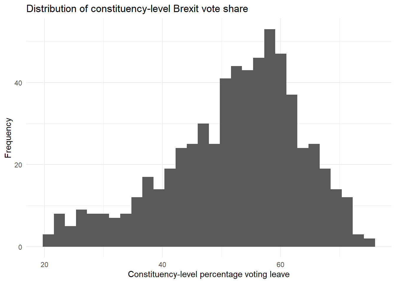

The percentage voting leave in different constituencies is quite clustered in 50-60%, but lots of constituencies also had leave vote shares lower than 50%, and some had vote shares higher than 60%.

Our binary independent variable is London which tells us whether a constituency is in London or not. Let’s look at how it is distributed.

london_bar <- ggplot(data = brexit, aes(London)) +
  geom_bar() +
  labs(x = "Constituency location",
       y = "Frequency",
       title = "Number of constituencies inside and outside of London") +
  theme_minimal()

london_bar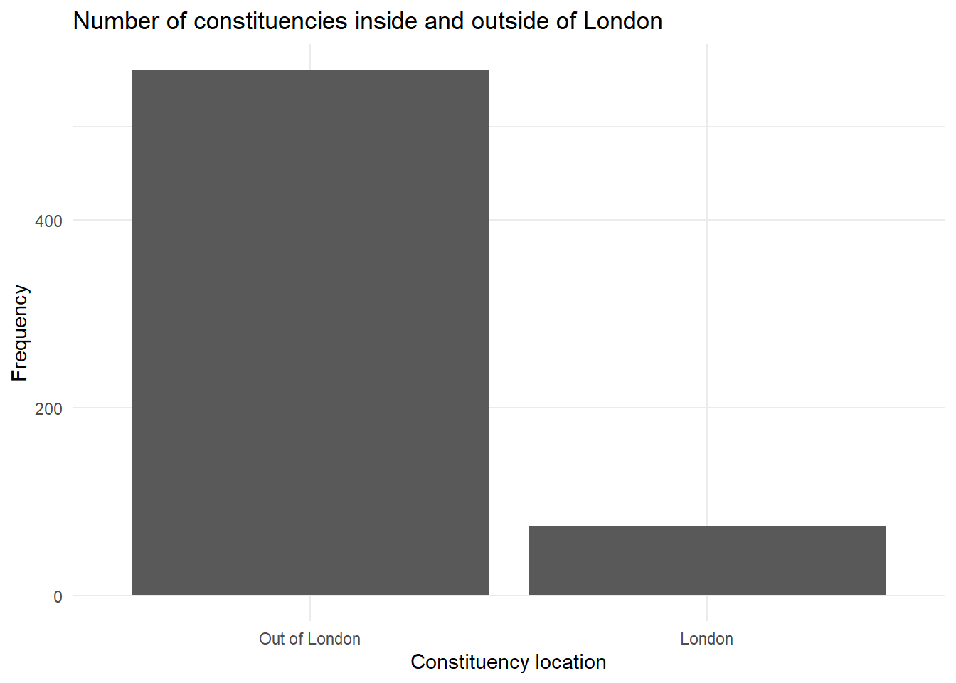

As we would expect, the vast majority of constituencies are not considered to be in London.

Let’s check the summary statistics of our dependent variable BrexitVote using summary().

summary(brexit$BrexitVote)

   Min. 1st Qu.  Median    Mean 3rd Qu.    Max. 
  20.54   45.39   53.74   52.07   60.14   74.96

Someone claims that constituencies in London were less likely to vote to leave overall. From the output of the summary() fucntion, we know that average support for leave is 52.07271% across all constituencies — those in and outside of London.

We want to get the mean of BrexitVote for each location of constituency individually. There are several ways to do this. The tidyverse has a nice option using group_by() and summarise(), building on what we have done in previous weeks.

# tidyverse grouped means 

brexit_means <- # assign to object
  brexit %>% # pipe dataset
  group_by(London) %>% # group by whether in London
  summarise(mean = mean(BrexitVote), # get mean of BrexitVote for each group
            n = n()) # also get number of observations in each group

brexit_means

# A tibble: 2 x 3
  London         mean     n
  <fct>         <dbl> <int>
1 Out of London  53.6   559
2 London         40.2    73

It definitely looks like there is a meaningful difference between London and non-London constituencies. We can run a t-test to check if this difference is statistically significant.

We use formula syntax to see how our dependent variable (here BrexitVote) varies between the levels of our independent variable (here London). The dependent variable goes before a tilde (~) and the independent variable comes after. So what we are doing here is taking a continuous variable and comparing its means in different groups of a binary nominal variable to see if there is a significant, systematic difference between those groups.

t.test(BrexitVote ~ London, # formula y ~ x
       data = brexit, # dataset where the variables are found
       mu = 0, # difference under the null hypothesis
       alt = "two.sided",  # two sided test (difference in means could be smaller or larger than 0)
       conf = 0.95) # confidence interval


    Welch Two Sample t-test

data:  BrexitVote by London
t = 8.3366, df = 83.455, p-value = 1.338e-12
alternative hypothesis: true difference in means is not equal to 0
95 percent confidence interval:
 10.23275 16.64471
sample estimates:
mean in group Out of London        mean in group London 
                   53.62497                    40.18624

Let’s interpret the results you get from t.test(). The first line tells us which groups we are comparing. In our example: Do constituencies in London have different average vote shares for leave compared to those outside of London?

In the following line you see the t-value, the degrees of freedom and the p-value. Knowing the t-value and the degrees of freedom you can check in a table on t distributions how likely you were to observe this data, if the null-hypothesis were true. The p-value gives you this probability directly. For example, a p-value of 0.02 would mean that the probability of seeing this data given that there is no difference in average support for leave in the population, is 2%. Here the p-value is much smaller than this: 1.338e-12 = 0.000000000001338!

In the next line you see the 95% confidence interval because we specified conf=0.95. If you were to take 100 samples and in each you checked the means of the two groups, 95 times the difference in means would be within the interval you see there.

At the very bottom you see the means of the dependent variable by the two groups of the independent variable. These are the means that we estimated above. In our example, you see the mean Brexit vote share in constituencies in London, and in constituencies outside of London.

Furthermore, note that in the t test for the differences in means, the degrees of freedom depend on the variances in each group. You do not have to compute degrees of freedom for t tests for the differences in means yourself in this class — just use the t.test() function.

6.1.2.1 Another example t-test

We might have other theories about how support for leave varies by different types of constituency. For example, we might hypothesise that it’s not necessarily being in London or not that matters, but rather how densely populated a constituency is. We could argue that more densely populated constituencies are more likely to be urban environments where people were less likely to vote to leave. Currently our population density variable is continuous, and we can see how it is distributed. This time, let’s look at it as a boxplot.

pop_box <- ggplot(brexit, aes(PopulationDensity)) + 
  geom_boxplot() + # create boxplot
  theme_minimal() +
  coord_flip() + # make it vertical
  theme(axis.text.x = element_blank()) # remove meaningless axis text

pop_box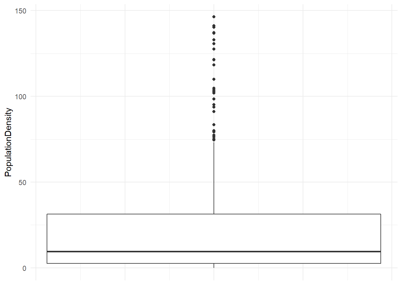

As we can see, most constituencies are not particularly densely populated, with far fewer than 50 people per square mile. You can scrutinise this boxplot more closely using your knowledge of what each part of the plot means.

We can’t use a continuous variable like this as our independent variable in a t-test. For this we need a binary indicator or dummy variable. We can create a variable which tells us whether a constituency has higher than median population density.

# calculate median population density
med_dens <- median(brexit$PopulationDensity)

# create new variable using case_when()
brexit <- brexit %>% # pipe the dataset
  mutate( # create new variable
    density_dummy = # name the new variable
      factor(case_when(
        PopulationDensity > med_dens ~ 1,
        PopulationDensity <= med_dens ~ 0)))

We can get an idea of whether the distribution of support for leave differs by this new variable by plotting the conditional distribution.

density_dist <- ggplot(data = brexit, aes(BrexitVote, group = density_dummy)) + 
  geom_density(aes(colour = density_dummy)) +
  labs(x = "Vote share for leave in Brexit referendum", # clearer x axis label
       y = "Density", # clearer y axis label
       title = "Distribution of Brexit vote share conditional on population density") + # title 
  scale_color_discrete(name = "Population density", # change legend title
                       labels = c("Below or equal median", # change legend labels
                                  "Above median")) + 
  theme_minimal()

density_dist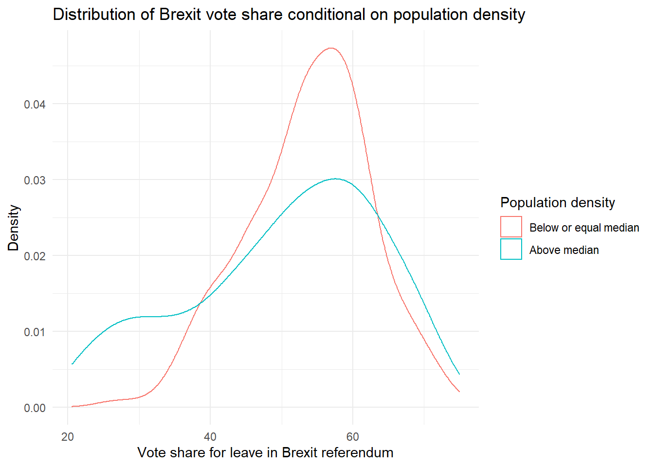

The distributions are quite different, and those constituencies with above-average population densities seem to have a wider spread of Brexit vote shares in general. Beyond that, though, it is difficult to tell if the mean level of support for leave will differ considerably across the two groups.

We can now run a t-test to check this.

t.test(BrexitVote ~ density_dummy, # formula y ~ x
       data = brexit, # dataset where the variables are found
       mu = 0, # difference under the null hypothesis
       alt = "two.sided",  # two sided test (difference in means could be smaller or larger than 0)
       conf = 0.95) # confidence interval


    Welch Two Sample t-test

data:  BrexitVote by density_dummy
t = 3.7724, df = 540.65, p-value = 0.0001795
alternative hypothesis: true difference in means is not equal to 0
95 percent confidence interval:
 1.625877 5.158793
sample estimates:
mean in group 0 mean in group 1 
       53.76888        50.37654

Overall, it does seem to be the case that more densely populated constituencies voted to leave at lower rates on average. The difference in means is only a few percentage points, but this difference is highly statistically significant.

6.1.3 Exercises

Follow the equivalent steps to those we took above to find the means of Brexit vote share in constituencies that (1) have higher than average number of citizens who were born in the UK, (2) those equal to the median or lower in terms of numbers of UK-born citizens.
Create a conditional distribution plot to visualise how the distribution of Brexit vote share differs in these two groups of constituencies.
Run a t-test to see if the difference in means statistically significant at an alpha level of 0.05. What about 0.01?