Chapter 5 Sampling distribution of the mean, confidence intervals, and significance
5.1 Seminar
When doing research, we rarely have data on full populations. We often only have sample data. If we wanted to know, for example, the average age level of the criminal and non-criminal population of Camden it would be impractical to collect data on every person in the borough. So we might survey a sample, or subset, of this population. But, how can we be sure our sample estimate is correct, and would we get a different estimate if we selected a different sample?
For this and similar problems we need to apply statistical inference. We want to learn something about the population by looking at a smaller sample of it. Statistical inference provides a set of tools that allow us to draw inferences from sample data in this way. Unlike in previous and future seminars, the focus this week will be less applied and a bit more theoretical. However, the foundations of statistical inference are essential for a proper understanding of everything else we cover in this module.
We are going to need the tidyverse, so make sure it is loaded!
# don't have tidyverse installed? Run:
# install.packages('tidyverse')

# load tidyverse
library(tidyverse)
5.1.1 Generating ramdom data
For the purpose of this week’s sessions we are going to generate some fictitious data. We use real data in other tutorials but it is convenient for this session to have some randomly generated fake data.
So that all of us gets the same results (otherwise there would be random differences!), we need to use the set.seed(). Doing this guarantees that all of us get the same randomly generated numbers:
set.seed(100)We are going to generate an object with skewed data using the rnbinom() function for something called negative binomial distributions. Don’t worry too much about what this means. Basically, data isn’t always distributed ‘normally’, but can take on lots of differently shaped distributions. When we want to try things out on fake data, we can use these different distributions to create data which is distributed in different ways, which might reflect how we would expect equivalent real-world data to be distributed.
# Creates vector of negative binomial distributed data
skewed <- rnbinom(100000,
                  mu = 0.5,
                  size = 0.1)
We can get the mean and standard deviation for this object.
mean(skewed)[1] 0.49996sd(skewed)[1] 1.726659And we can also see how it looks, using qplot() from ggplot2(). This function is useful if you want to quickly display the distribution of an object that is not in a data.frame. This can also be done in a ggplot() call. Note that ggplot2() should have been automatically loaded when we loaded the tidyverse earlier on. We can still run library(ggplot2) if we want, just to check!
# make sure ggplot2 is loaded
library(ggplot2)

# plot distribution
qplot(skewed) +
  theme_minimal() +
  labs(x = "Number of crimes committed",
       y = "Frequency in data")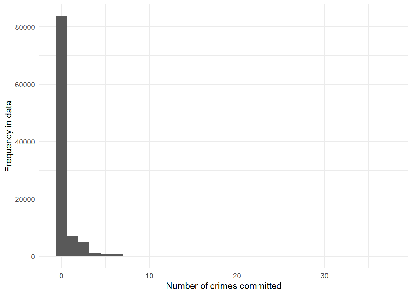
# alternative using ggplot()
ggplot(mapping = aes(skewed)) +
  geom_histogram() +
  theme_minimal() +
  labs(x = "Number of crimes committed",
       y = "Frequency in data")
We are going to pretend this variable measures the number of crimes perpetrated by every individual in Camden in 2019. We are assuming there are 100,000 people in Camden, so this data represents the full population. Let’s see how many offenders we have.
sum(skewed > 0)[1] 16422From the distribution we plotted above, we can see that the vast majority of people committed precisely zero crimes. Most people obey the law! We might actually expect, in the real world, an even larger proportion of zeroes. As it is, 16422 of our 100,000 Camden residents committed one or more crimes in 2019.
We are now going to put this variable in a dataframe and create a new categorical variable identifying whether someone offended over the past year (e.g., anybody with a count of crime higher than 0). Variables like this, which take a value of either 0 or 1, are also called ‘dummy’ or ‘binary’ variables. We are going to create this variable using a piped mutate() – hopefully you will remember the introduction to this in Week 4’s seminar!
# create dataframe with our data as one column
fake_population <- data.frame(crime = skewed)

# create 'offender' variable - dummy indicator of whether someone has committed one or more crimes, rather than zero
fake_population <- fake_population %>% # load and pipe dataset
  mutate(
    offender = factor(
      case_when( # create new factor variable following certain conditions
        crime > 0 ~ 1, # value of 1 if crimes committed greater than zero
        TRUE ~ 0 # value of 0 otherwise
  )))

# Let's check the results
table(fake_population$offender)
    0     1
83578 16422
We are now going to generate a normally distributed variable which we will pretend measures our respondents’ age, in years, in 2019. We are going to assume that this variable has a mean of 30 in the non-criminal population with a standard deviation of 10 and a mean of 20 with a standard deviation of 4 in the criminal population. This fits the observation that ‘studies have unanimously concluded that such [criminal] behavior is most heavily concentrated in the second and third decades of life’ (Ellis, Beaver, and Wright 2009). We should find that most of the offenders in our dataset are in their teens or twenties, while non-offenders’ ages are more dispersed. The number of datapoints we ask for rnorm() to give us reflects the numbers in the table above. We use nrow(.) here to get the correct number of age values in each case without needing to type out the number manually.
# create age variable depending on committing crime or not

# subset to offenders, create age
offenders <- fake_population %>% # pipe dataset
  filter(offender == 1) %>% # subset to offenders
  mutate(age = round(rnorm(nrow(.),
                     mean = 20,
                     sd = 4))) # random numbers from normal distribution rounded to whole numbers

# subset to non-offenders, create age
non_offenders <- fake_population %>% # pipe dataset
  filter(offender == 0) %>% # subset to non-offenders
  mutate(age = round(rnorm(nrow(.),
                     mean = 30,
                     sd = 10))) # random numbers from normal distribution rounded to whole numbers

# bring both subsets back together
fake_population <- rbind(offenders,
                         non_offenders)
We can now have a look at the data. Let’s plot the density of age for each of the two groups and have a look at the summary statistics.
# average age across all respondents
mean(fake_population$age)
[1] 28.36027# dataset of means for each group independently
age_means <- fake_population %>% # pipe dataset
group_by(offender) %>% # group so that function can be applied to offenders and non-offenders separately
summarise(age = mean(age)) # get mean of each group# plot
gg_age_crimes <- ggplot(fake_population,
aes(x = age,
group = factor(offender),
colour = offender)) +
geom_density() +
geom_vline(data = age_means,
mapping = aes(xintercept = age, colour = offender),
linetype = "dashed", size = 1) +
theme_minimal() +
labs(title = "Distribution of age conditional on offender status",
x = "Age in 2019",
y = "Density") +
scale_colour_discrete(name = "Committed crime in 2019",
labels = c("No", "Yes"))
gg_age_crimes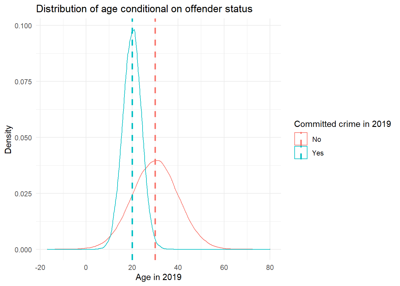
So, now we have our fake population data. In this case, because we generated the data ourselves, we know what the population data looks like and we know what the summary statistics for the various attributes (age, crime) of the population are. But in real life we don’t normally have access to full population data. It is for this reason we rely on samples.
5.1.2 Sampling data and sampling variability
It is fairly straightforward to sample data with R. The following code shows you how to obtain a random sample of size 10 from our population data above:
# get 10 values of age
sample(fake_population$age, 10)
[1] 30 18 31 20 33 32 32 34 25 11You may be getting different results, depending on the seed you used and how many times before you tried to obtain a random sample. You can compute the mean for a sample generated this way:
mean(sample(fake_population$age, 10))[1] 27.6And every time you do this, you will be getting a slightly different mean. This is one of the problems with sample data. No two samples are going to be exactly the same and as a result, every time you compute the mean you will be getting a slightly different value. Run the function three or four times and notice the different means you get.
5.1.3 Sampling distributions and sampling experiments
A sampling distribution is the probability distribution of a given statistic based on a random sample. It may be considered as the distribution of the statistic for all possible samples from the same population of a given size.
We can have a sense for what the sampling distribution of the means of age for samples of size 10 in our example by taking a large number of samples from the population.
# take 20000 samples of the age mean - may take a bit of time!
sampd_age_10 <- replicate(20000, mean(sample(fake_population$age, 10)))

# compute the mean of this sampling distribution of the means and compare it to the population mean

mean(sampd_age_10) # mean of the sample means
[1] 28.35146mean(fake_population$age) # mean of the population[1] 28.36027What we have observed is part of something called the central limit theorem, a concept from probability theory. One of the first things that the central limit theorem tells us is that the mean of the sampling distribution of the means (also called the expected value) should equal the mean of the population. So, if we take a huge amount of samples from the population, the mean of the means of each of those samples will tend towards the population mean. It won’t be quite the same in this case (to several decimal places, anyway) because we only took 20000 samples, but in the very long run (if you take many more samples) they would be the same.
Let’s now visually explore the distribution of the sample means.
# plot the means
qplot(sampd_age_10,
      xlab = "Distribution of means from samples of size 10") + # add x axis label
  theme_minimal()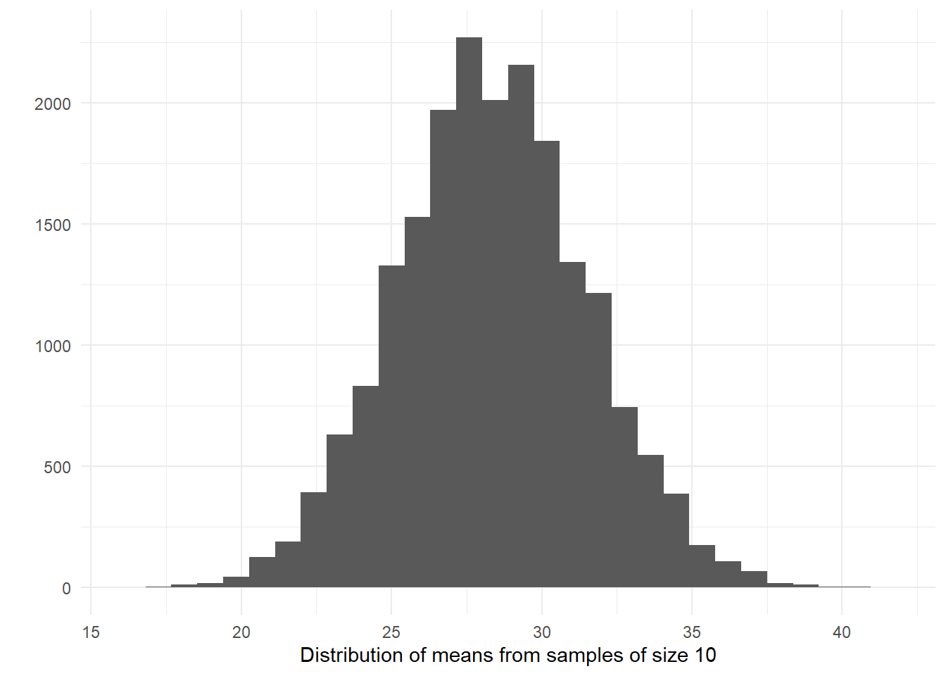
When you take many random samples from a normally distributed variables, compute the means for each of these samples, and plot the means of each of these samples, you end up with something that is also normally distributed. The sampling distribution of the means of normally distributed variables in the population is normally distributed.
What this type of distribution for the sample means is telling us is that most of the samples will give us guesses that are clustered around their own mean, as long as the variable is normally distributed in the population (which is something, however, that we may not know). Most of the sample means will cluster around the value of 28.36 (in the long run). There will be some samples that will give us much larger and much smaller means (look at the right and left tail of the distribution), but most of the samples won’t gives us such extreme values.
Another way of saying this is that the means obtained from random samples behave in a predictable way. When we take just one sample and compute the mean we won’t be able to tell whether the mean for that sample is close to the centre of its sampling distribution. But we will know the probability of getting an extreme value for the mean is lower than the probability of getting a value closer to the mean. That is, if we can assume that the variable in question is normally distributed in the population.
Let’s repeat the exercise with a sample size of 30, 100 and 1000.
sampd_age_30 <- replicate(20000, mean(sample(fake_population$age, 30)))
sampd_age_100 <- replicate(20000, mean(sample(fake_population$age, 100)))
sampd_age_1000 <- replicate(20000, mean(sample(fake_population$age, 1000)))

# plot different sampling distributions
p2 <- ggplot() +
  geom_density(aes(x = sampd_age_1000,
                   fill = "1000"),
               alpha = 0.4) + # alpha changes the transparency
  geom_density(aes(x = sampd_age_100,
                   fill = "100"),
               alpha = 0.4) +
  geom_density(aes(x = sampd_age_30,
                   fill = "30"),
               alpha = 0.4) +
  scale_fill_discrete(name = "Sample size", # legend title
                      limits = c("1000", "100", "30")) + # correct order of labels
  labs(x = "Distribution of mean value of age",
       y = "Density") +
  theme_minimal()

p2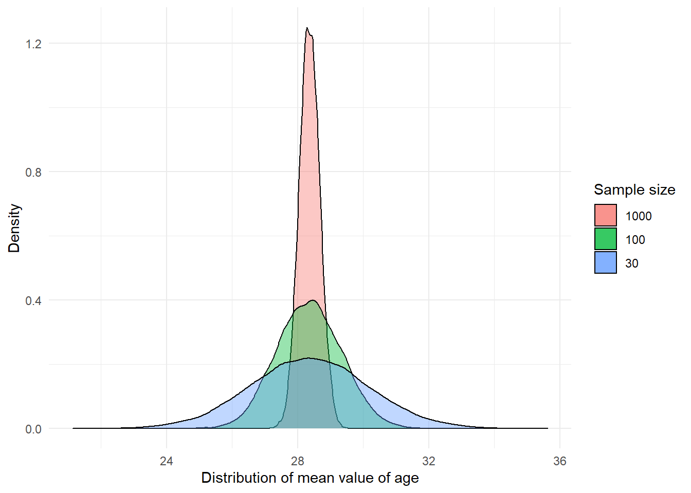
Notice the differences between these sampling distributions? As the sample size increases, more and more of the samples tend to cluster closely around the mean of the sampling distribution. In other words with larger samples the means you get will tend to differ less from the population mean than with smaller samples. You will be less likely to get means that are dramatically different from the population mean.
Let’s take a closer look at the summary statistics for each sample size:
summary(sampd_age_30) Min. 1st Qu. Median Mean 3rd Qu. Max.
21.13 27.13 28.37 28.36 29.57 35.63 summary(sampd_age_100) Min. 1st Qu. Median Mean 3rd Qu. Max.
24.89 27.67 28.35 28.35 29.02 32.37 summary(sampd_age_1000) Min. 1st Qu. Median Mean 3rd Qu. Max.
27.00 28.15 28.36 28.36 28.57 29.59 As you can see the mean of the sampling distributions is pretty much the same regardless of sample size, though since we only did 20000 samples there’s still some variability. But notice how the range (the difference between min and max) and the interquartile range (difference between 1st Qu and 3rd Qu) are much larger when we use smaller samples. When the sample size is smaller the range of possible means is wider and you are more likely to get sample means that are further from the expected value.
This variability is also captured by the standard deviation of the sampling distributions, which is smaller the larger the sample size is. The standard deviation of a sampling distribution receives a special name you need to remember: the standard error. In our example, with samples of size 30 the standard error is 1.81, whereas with samples of size 1000 the standard error is 0.31.
We can see that the precision of our guess or estimate improves as we increase the sample size. Using the sample mean as an estimate (we call it a point estimate because it is a single value, a single guess) of the population mean is not a bad thing to do if your sample size is large enough and the variable can be assumed to be normally distributed in the population. More often than not this guess won’t be too far off in those circumstances.
But what about variables that are not normally distributed? What about crime? We saw this variable was quite skewed. Let’s take numerous samples, compute the mean of crime, and plot its distribution.
sampd_CR_30 <- replicate(20000, mean(sample(fake_population$crime, 30)))
sampd_CR_100 <- replicate(20000, mean(sample(fake_population$crime, 100)))
sampd_CR_1000 <- replicate(20000, mean(sample(fake_population$crime, 1000)))


# plot results
p3 <- ggplot() +
  geom_density(aes(x = sampd_CR_1000, fill = "1000"),
               alpha = 0.4) +
  geom_density(aes(x = sampd_CR_100, fill = "100"),
               alpha = 0.4) +
  geom_density(aes(x = sampd_CR_30, fill = "30"),
               alpha = 0.4) +
  scale_fill_discrete(name = "Sample size",
                      limits = c("1000", "100", "30")) +
  xlab("Distribution of mean value of crime") +
  theme_minimal()
p3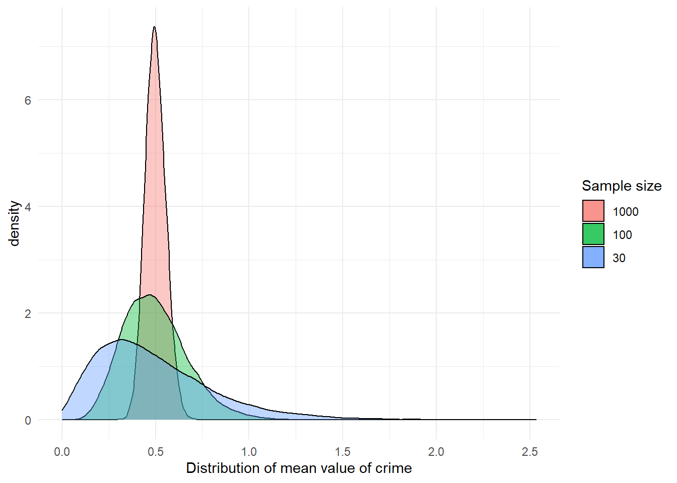
summary(sampd_CR_30) Min. 1st Qu. Median Mean 3rd Qu. Max.
0.0000 0.2667 0.4333 0.4938 0.6667 2.5333 summary(sampd_CR_100) Min. 1st Qu. Median Mean 3rd Qu. Max.
0.090 0.370 0.480 0.498 0.600 1.320 summary(sampd_CR_1000) Min. 1st Qu. Median Mean 3rd Qu. Max.
0.2970 0.4620 0.4970 0.4996 0.5360 0.7220 mean(fake_population$crime)[1] 0.49996You can see something similar happens, even though crime itself is not normally distributed. The sampling distribution of the means of crime becomes more normally distributed the larger the sample size gets. Although we are not going to repeat the exercise again, the same would happen even for the variable offender. With a binary categorical variable such as offender (remember it could take two values: yes or no) the mean represents the proportion with one of the outcomes. But essentially the same process applies.
What we have seen in this section is an illustration of various amazing facts associated with the central limit theorem. Most sample means are close to the population mean, very few are far away from the population mean, and on average, we get the right answer (i.e., the mean of the sample means is equal to the population mean). This is why statisticians say that the sample mean is an unbiased estimate of the population mean.
How is this helpful? Well, it tells us we need large samples if we want to use samples to guess population parameters without being too far off. It also shows that although sampling introduces error (sampling error: the difference between the sample mean and the population mean), this error behaves in predictable ways (in most of the samples the error will be small, but it will be larger in some: following a normal distribution).
If you want to further consolidate some of these concepts you may find these videos on sampling distributions from Khan Academy useful.
5.1.4 The normal distribution and confidence intervals with known standard errors
While the sample mean may be the best single number to use as an estimate of the population mean, particularly with large samples, each sample mean will continue to come with some sample error (with some distance from the population mean). How can we take into account the uncertainty in estimating the population mean that derives from this fact?
The key to solving the problem lies in the fact that the sampling distribution of the means will approach normality with large samples. If we can assume that the sampling distribution of the means is normally distributed then we can take advantage of the properties of the standard normal distribution.
One of the peculiarities of the standard normal distribution is that we know the proportion of cases that fall within standard deviation units away from the mean. In the graphic below you can see the percentage of cases that fall within one and two standard deviations from the mean in the standard normal distribution:
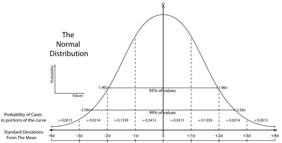
We know that the sampling distribution of the means can be assumed with large samples to have a shape like this. You can think of the sampling distribution of the means as the distribution of sampling error. Most sample means fall fairly close to the expected value (i.e., the population mean) and so have small sampling error. Many fall a moderate distance away. Just a few fall in the tails of the sampling distribution, which signals large estimation errors. So although working with sample data we don’t have a precise distance, we have a model that tells us how that distance behaves (i.e., it follows a normal distribution).
This is very useful because then we can use this knowledge to generate the margin of error. The margin of error is simply the largest likely sampling error. In social science we typically take ‘likely’ to imply 95%, so that there is a 95% chance that the sampling error is less than the margin of error. By extension this means that there is only a 5% chance that the sampling error will be bigger: that we have been very unlucky and our sample mean falls in one of the tails of the sampling distribution.
Looking at the standard normal distribution we know that about 95% of the cases fall within 1.96 standard deviations on either side of the mean. The margin of error equals 1.96 standard errors.
This may be clearer with an example. Let’s focus on our variable age. Look at the standard error (the standard deviation of the collection of sample means) for the sampling distribution of age when we took samples of 1000 cases. We produced this earlier on.
The standard error was 0.31. If we multiply 0.31 by 1.96 we obtain 0.61. This means that 95% of the cases in this sampling distribution will have an error that won’t be bigger than that. They will only at most differ from the mean of the sampling distribution by (plus and minus) 0.61. However, 5% of the samples will have a margin of error bigger than that (in absolute terms – positively or negatively).
Everyone will have different standard errors because the set seed function only works for the code immediately after it. Then, we all have different 20,000 samples from our fake population data.
We can use it to give a measure of the uncertainty in our estimation. If we have a large random sample, the 95% confidence interval will then be: Upper limit = sample mean + 1.96 standard error Lower limit = sample mean - 1.96 standard error
Let’s extract a sample of size 1000 from the fake_population and look at the distribution of age:
sample_1_age <- sample(fake_population$age, 1000)
mean(sample_1_age)
[1] 28.274When we then take the mean of age in this sample, we get the value in the above output. It does not matter if you get a different value. Remember the standard error for the sampling distribution of age when we took samples of 1000 cases. It was 0.31. If we multiply 0.31 times 1.96 we obtain 0.61. The upper limit for the your confidence interval will be your sample mean plus 0.61 (the margin of error) and the lower limit for the confidence interval will be your sample mean minus 0.61. This yields a confidence interval ranging from your lower limit to your upper limit. Calculate these values.
Now, if your sample mean had been different, your confidence interval would have also been different. If you take 10,000 sample means and compute 10,000 confidence intervals they will be different among themselves. In the long run, that is, if you take a large enough numbers of samples and then compute the confidence interval for each of the samples, 95% of those confidence intervals will capture the population mean and 5% will miss it. Let’s explore this.
# select 100 means (from the samples of size 1000) out of the 20,000 samples that we created
samp_age_100 <- sampd_age_1000[1:100]
ci_age <- data.frame(mean_age = samp_age_100)
We are now going to create the lower and the upper limit for the CI.
First we obtain the margin of error. To do this we will compute the summary statistics for the sampling distribution and then multiply the standard error (e.g., the sd of the sampling distribution) times 1.96.
We have 100 random numbers. These could be taken as the ages of 100 different people (one sample of n=100 distribution) or as the means of 100 different samples (sampling distribution). For the first one, we could use the se estimate as R assumes that it is one sample. For the second one we need to use the sd estimate, which is the proper definition of SE (standard deviation of the sampling distribution).
# get standard error which is just the sd of the sampling dist
se_sampd_age_100 <- sd(ci_age$mean_age)

# times by 1.96 for the margin of error
me_age_100 <- se_sampd_age_100 * 1.96

# create two numerical vectors with the upper and the lower limit, adding them to the data frame we created
ci_age$LowerLimit <- samp_age_100 - me_age_100
ci_age$UpperLimit <- samp_age_100 + me_age_100
You may want to use the View() function to see inside the ci_age data frame that we have created. Every row represents a sample and for each sample we have the mean and the limits of the confidence interval. We can now query how many of these confidence intervals include the mean of the variable age in our fake population data.
# create logical (TRUE/FALSE) vector by providing conditions to satisfy
ci_age$contains_mean <-
  (ci_age$LowerLimit <= mean(fake_population$age)) & # lower limit is less than or equal to mean
  (ci_age$UpperLimit >= mean(fake_population$age)) # upper limit is greater than or equal to mean

sum(ci_age$contains_mean) # how many are true, out of 100?
[1] 94Thus 94 intervals contain the true population mean. As there are 100 intervals, this means 94 % of them contain the true population mean. This should hold with different numbers of intervals - the figure should generally stay very close to 95%. Here, you probably got a number just below 95%. What do you think that suggests to us about using a sample size of 1000 in the current study?
We can also plot these confidence intervals. First, let’s make a unique variable to identify each row by. This helps with plotting.
# rowname is by default a unique number
ci_age$id <- rownames(ci_age)
We are going to use a new geom to create lines with a point in the middle. You need to tell R where the line begins and ends, as well as where to locate the point in the middle. The point in the middle is our mean and the lines range from the lower limit and upper limit. Each line represents the confidence interval. Often these are called ‘dot and whisker’ plots. We will use the ID variable so that R plots one line for each of the samples. Finally we’ll use the contains_mean variable to clearly distinguish the CIs that cover the population mean.
geom_hline()will create a horizontal line representing the population mean, so that we can clearly see itscale_x_discrete()ensures that no tick marks and labels are used in the axis defining each sample (run code without this line to see what happens)
p4 <- ggplot(ci_age, aes(x = id, # each unique case on x axis (flipped later)
                        y = mean_age, # the sample mean on y axis (flipped later)
                        colour = contains_mean)) + # colour depends on if range covers population mean
  # first create a clear solid line at the population mean
  geom_hline(yintercept = mean(fake_population$age), colour="red", size=1) +
  # next create a pointrange geom in which point is mean and lines go from lower to upper limit
  geom_pointrange(aes(ymin = LowerLimit,
                      ymax = UpperLimit)) +
  # change theme to make colours clearer
  theme_bw() +
  # set plot title
  ggtitle("CIs for the mean (100 samples of size 100)") +
  # change axis and legend labels
  labs(colour="Covers µ?", x = "", y ="Mean of age") +
  # remove axis ticks for each case
  scale_x_discrete(breaks = "") +
  # flip coordinates (x becomes y, vice versa)
  coord_flip()

p4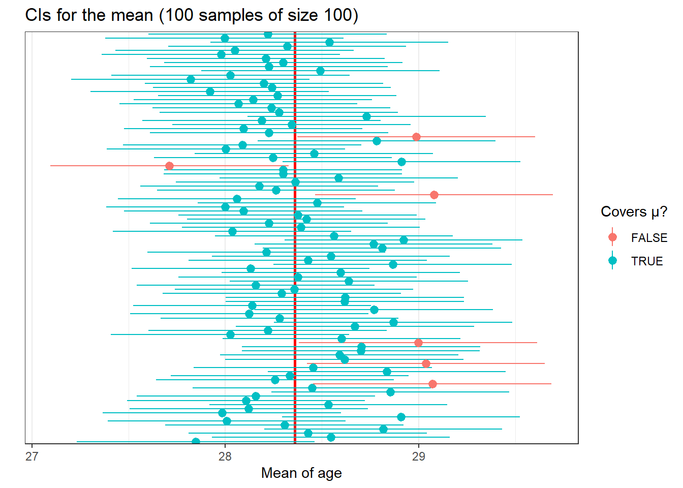
As you can see, most of the confidence intervals cover the population mean, but sometimes this does not happen. If you know the population mean, then you can see whether that happens or not. But in real life we run samples because we don’t know the population parameters. So, unfortunately, when you do a sample you can never be sure whether your estimated confidence interval is one of the red or the blue ones. The truth is we will never know whether our confidence interval captures the population parameter or not, we can only say that under certain assumptions if we had repeated the procedure many times it will include it 95% of the time. This is one of the reasons why in statistics, when making inferences, we cannot provide definitive answers.
It is, however, better to report your confidence intervals (CI) than your point estimates. Why? Because you are being explicit about the fact you are just guessing. Point estimates such as the mean create a false impression of precision.
But beware the CI can also be misleading! If we take multiple samples from our population (where each sample mean has its own confidence interval), 95% of the times these confidence intervals will include the true population mean. This is the meaning of a confidence interval, and not the meanings some applied statisticians give it.
CI is worth reporting also because, if the range of values that you give for your CI is smaller or bigger, we will know that your estimate is more or less precise respectively. That is, with the CI you are giving me a measure of your uncertainty. The bigger the CI the more uncertain we are about the true population parameter.
5.1.5 Confidence intervals for means and proportions using t-distribution in R
You may have spotted that the computation of the confidence intervals requires that we know the standard error of the sampling distribution of the mean. How did we compute the confidence interval? We multiplied 1.96 times the standard error. Remember: the standard error is the standard deviation of the sampling distribution of the mean. This is rarely known and we are often required to estimate confidence intervals using data from a sample.
You can use the standard deviation of your sample to estimate the standard error when you have a large enough sample size (>100). For small samples, we use a different distribution that is flatter and has greater variance: a t-distribution. It is fairly straightforward to get the confidence intervals using a t-distribution in R. In order to use the t distribution we need to assume the data were randomly sampled and that the population distribution is unimodal and symmetric. That is, it basically looks like a normal distribution.
Earlier we created a sample of 100 cases from our fake population. Let’s build the confidence intervals using the sample standard deviation as an estimate for the standard error and assuming we can use the t-distribution:
t.test(sample_1_age)
    One Sample t-test

data:  sample_1_age
t = 85.827, df = 999, p-value < 2.2e-16
alternative hypothesis: true mean is not equal to 0
95 percent confidence interval:
 27.62754 28.92046
sample estimates:
mean of x
   28.274
Ignore for now the few first lines. Just focus on the 95% interval. You will see it is not wildly different from the one we derived using the actual standard error.
If you want a different confidence interval, say 99%, you can pass an additional argument to change the default in the t.test() function:
t.test(sample_1_age, conf.level = .99)
    One Sample t-test

data:  sample_1_age
t = 85.827, df = 999, p-value < 2.2e-16
alternative hypothesis: true mean is not equal to 0
99 percent confidence interval:
 27.42382 29.12418
sample estimates:
mean of x
   28.274
We will talk more about t-tests next week.
What if you have a factor variable (i.e. nominal or categorical) and want to estimate a confidence interval for a proportion? In our data we have a dummy (0,1) variable that identifies cases as offenders. Let’s extract a sample of size 100 from the fake_population and look at the distribution of offender:
sample_1_offender <- sample(fake_population$offender, 100)

table(sample_1_offender)
sample_1_offender
0 1
84 16 We can use the prop.test() function from mosaic in these cases:
# get and load mosaic package
install.packages('mosaic', repos = 'http://cran.us.r-project.org')library(mosaic)
mosaic::prop.test((sample_1_offender))
    1-sample proportions test with continuity correction

data:  (  [with success = 0]sample_1_offender  [with success = 0]
X-squared = 44.89, df = 1, p-value = 2.084e-11
alternative hypothesis: true p is not equal to 0.5
95 percent confidence interval:
 0.7501478 0.9030053
sample estimates:
   p
0.84
You can also specify a different confidence level:
mosaic::prop.test((sample_1_offender), conf.level = .99)
    1-sample proportions test with continuity correction

data:  (  [with success = 0]sample_1_offender  [with success = 0]
X-squared = 44.89, df = 1, p-value = 2.084e-11
alternative hypothesis: true p is not equal to 0.5
99 percent confidence interval:
 0.7192513 0.9163248
sample estimates:
   p
0.84
5.1.6 Exercises
Try to the following questions using complete sentences. Take this as a practice for the midterm assessment. It might be easier to calculate the results you need using R.
- You sample 120 people and measure their blood pressure before and after an intervention and find that the mean change is -5.09 with a standard deviation of 16.71. Find the 95% and 99% confidence intervals of the mean change. Does the intervention reduce blood pressure in the population?
- In the same sample of 120 people you find that 61% showed a decrease in blood pressure. Find the 95% and 99% confidence intervals of the proportion. Does this confirm the effect of the intervention on blood pressure? Note that in this case you need to estimate the standard error of a proportion.
- A random sample of 25 countries finds that the mean life expectancy is 64 years for women with a standard deviation of 21 years and 62 years for men with a standard deviation of 14 years. Using a t-distribution, find the 95% and 99% confidence intervals of the mean for men and for women. Interpret your results.