Chapter 2 Getting to Know Your Data: Central Tendency and Dispersion
2.1 Seminar
In today’s seminar, we work with measures of central tendency and dispersion. You will learn more about these concepts in next week’s lecture, but we introduce them here because they are fundamental to how we describe data.
2.1.1 Central Tendency
Central tendency is a way of understanding what is a typical value of a variable – what happens on average, or what we would expect to happen if we have no information to give us further clues. For example, what is the average age of people in the UK? Or, what level of education does the average UK citizen attain? Or, are there more men or women in the UK?
The appropriate measure of central tendency depends on the level of measurement of the variable: continuous, ordinal or nominal.
| Level of measurement | Appropriate measure of central tendency |
|---|---|
| Continuous | arithmetic mean (or average) |
| Ordinal | median (or the central observation) |
| Nominal | mode (the most frequent value) |
2.1.1.1 Mean
Imagine eleven students take a statistics exam. We want to know about the central tendency of these grades. This is a continuous variable, so we want to calculate the mean. The mean is the arithmetic average: all of the results summed up, and divided by the number of results.
R is vectorised. This means that often, rather than dealing with individual values or data points, we deal with a series of data points that all belong to one ‘vector’ based on some connection. For example, we could create a vector of all the grades the students got in the exam. We create our vector of eleven (fake) grades using the c() function, where c stands for ‘collect’ or ‘concatenate’:
grades <- c(80, 90, 85, 71, 69, 85, 83, 88, 99, 81, 92)We can then do things to this vector as a whole, rather than to its individual components. R will do this automatically when we pass the vector to a function, because it is a vectorised coding language. All ‘vector’ means is a series of connected values like this. (A ‘list’ of values, if you like, but ‘list’ has a different, specific meaning in R, so we should really avoid that word here.)
We now take the sum of the grades.
sum_grades <- sum(grades)We also take the number of grades
number_grades <- length(grades) The mean is the sum of grades over the number of grades.
sum_grades / number_grades[1] 83.90909R provides us with an even easier way to do the same with a function called mean().
mean(grades)[1] 83.90909Remember that grades is an object we created by assigning the vector c(80, 90, 85, 71, 69, 85, 83, 88, 99, 81, 92) to the name ‘grades’ using the assignment operator <-. If this is unclear, take another look at Seminar 1.
2.1.1.2 Sequences
When creating vectors, we will often specifically need to create sequences. For instance, you might want to perform an operation on the first 10 rows of a dataset so we need a way to select the range we’re interested in. Typing out all of the individual values in a sequence can be cumbersome, so R gives us some simple shortcuts.
There are two ways to create a sequence. Let’s try to create a sequence of numbers from 1 to 10 using the two methods:
- Using the colon
:operator. If you’re familiar with spreadsheets then you might’ve already used:to select cells, for exampleA1:A20. In R, you can use the:to create a sequence in a similar fashion:
1:10 [1] 1 2 3 4 5 6 7 8 9 10- Using the
seqfunction we get the exact same result:
seq(from = 1, to = 10) [1] 1 2 3 4 5 6 7 8 9 10The seq function has a number of options which control how the sequence is generated. For example to create a sequence from 0 to 100 in increments of 5, we can use the optional by argument. Notice how we wrote by = 5 as the third argument. It is a common practice to specify the name of argument when the argument is optional. The arguments from and to are not optional, se we can write seq(0, 100, by = 5) instead of seq(from = 0, to = 100, by = 5). Both, are valid ways of achieving the same outcome. You can code whichever way you like. We recommend to write code such that you make it easy for your future self and others to read and understand the code.
seq(from = 0, to = 100, by = 5) [1] 0 5 10 15 20 25 30 35 40 45 50 55 60 65 70 75 80 85 90
[20] 95 100Another common use of the seq function is to create a sequence of a specific length. Here, we create a sequence from 0 to 100 with length 9, i.e., the result is a vector with 9 elements.
seq(from = 0, to = 100, length.out = 9)[1] 0.0 12.5 25.0 37.5 50.0 62.5 75.0 87.5 100.0Now it’s your turn:
- Create a sequence of odd numbers between 0 and 100 and save it in an object called
odd_numbers
odd_numbers <- seq(1, 100, 2)- Next, display
odd_numberson the console to verify that you did it correctly
odd_numbers [1] 1 3 5 7 9 11 13 15 17 19 21 23 25 27 29 31 33 35 37 39 41 43 45 47 49
[26] 51 53 55 57 59 61 63 65 67 69 71 73 75 77 79 81 83 85 87 89 91 93 95 97 99What do the numbers in square brackets
[ ]mean? Look at the number of values displayed in each line to find out the answer.Use the
lengthfunction to find out how many values are in the objectodd_numbers.- HINT: Try
help(length)and look at the examples section at the end of the help screen.
- HINT: Try
length(odd_numbers)[1] 502.1.1.3 Median
The median is the appropriate measure of central tendency for ordinal variables. Ordinal means that there is a rank ordering but not equally spaced intervals between values of the variable. Education is a common example. In education, more education is generally better. But the difference between primary school and secondary school is not the same as the difference between secondary school and an undergraduate degree. If you have only been to primary school, the difference between you and someone who has been to secondary school is probably going to be larger than the difference between someone who has been to secondary school and someone who has an undergraduate degree.
Let’s generate a fake example with 100 people. We use numbers to code different levels of education.
| Code | Meaning | Frequency in our data |
| 0 | no education | 1 |
| 1 | primary school | 5 |
| 2 | secondary school | 55 |
| 3 | undergraduate degree | 20 |
| 4 | postgraduate degree | 10 |
| 5 | doctorate | 9 |
We introduce a new function to create a vector. The function rep() replicates elements of a vector. Its arguments are the item x to be replicated and the number of times to replicate. Below, we create the variable education with the frequency of education level indicated above. Note that the arguments x = and times = do not have to be written out, but it is often a good idea to do this anyway, to make your code clear and unambiguous.
edu <- c( rep(x = 0, times = 1),
          rep(x = 1, times = 5),
          rep(x = 2, times = 55),
          rep(x = 3, times = 20),
          rep(4, 10), rep(5, 9)) # works without 'x =', 'times ='
The median level of education is the level where 50 percent of the observations have a lower or equal level of education and 50 percent have a higher or equal level of education. That means that the median splits the data in half.
We use the median() function for finding the median.
median(edu)[1] 2The median level of education is secondary school.
2.1.1.4 Mode
The mode is the appropriate measure of central tendency if the level of measurement is nominal. It is the most common value. Nominal means that there is no ordering implicit in the values that a variable takes on. We create data from 1000 (fake) voters in the United Kingdom who each express their preference on remaining in or leaving the European Union. The options are leave or stay. Leaving is not greater than staying and vice versa (even though we all order the two options normatively).
| Code | Meaning | Frequency in our data |
| 0 | leave | 509 |
| 1 | stay | 491 |
stay <- c(rep(0, 509),
          rep(1, 491))
The mode is the most common value in the data. There is no mode function in R. The most straightforward way to determine the mode is to use the table() function. It returns a frequency table. We can easily see the mode in the table. As your coding skills increase, you will see other ways of recovering the mode from a vector.
table(stay)stay
0 1
509 491 The mode is leaving the EU because the number of ‘leavers’ (0) is greater than the number of ‘remainers’ (1).
2.1.2 Dispersion
Central tendency is useful information, but two very different sets of data can have the same central tendency value while looking very different overall, because of different levels of dispersion. Dispersion describes how much variability around the central tendency there is in a variable or dataset.
The appropriate measure of dispersion again depends on the level of measurement of the variable we wish to describe.
| Level of measurement | Appropriate measure of dispersion |
|---|---|
| Continuous | variance and/or standard deviation |
| Ordered | range or interquartile range |
| Nominal | proportion in each category |
2.1.2.1 Variance and standard deviation
Both the variance and the standard deviation tell us how much an average realisation of a variable differs from the mean of that variable. So, they essentially tell us how much, on average, our observations differ from the average observation.
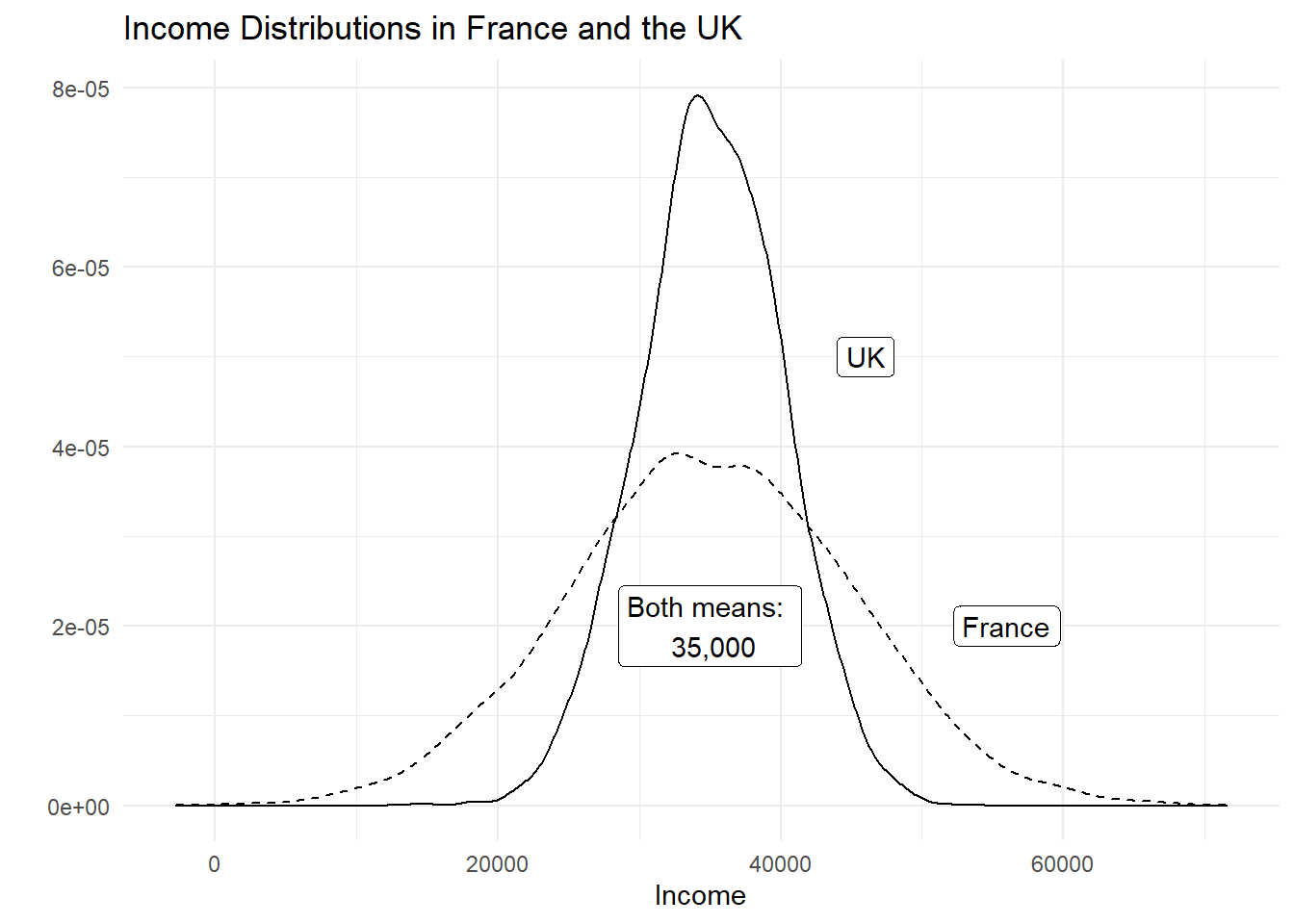
Let’s assume that our variable is income in the UK. Let’s assume that its mean is £35,000 per year. We also assume that the average deviation from £35,000 is £5,000. If we ask 100 people in the UK at random about their income, we get 100 different answers. If we average the differences betweeen the 100 answers and £35,000, we would get £5,000. Suppose that the average income in France is also £35,000 per year but the average deviation is £10,000 instead. This would imply that income is more equally distributed in the UK than in France, even though on average people earn around the same amount.
Dispersion is important to describe data, as this example illustrates. Although mean income in our hypothetical example is the same in France and the UK, the distribution is tighter in the UK. The figure below illustrates our example:
The variance gives us an idea about the variability of the data. The formula for the variance in the population is \[ \frac{\sum_{i=1}^n(x_i - \mu_x)^2}{n}\]
The formula for the variance in a sample adjusts for sampling variability, i.e., uncertainty about how well our sample reflects the population by subtracting 1 in the denominator. Subtracting 1 will have next to no effect if n is large but the effect increases the smaller \(n\) is. The smaller \(n\) is, the larger the sample variance. The intuition is, that in smaller samples, we are less certain that our sample reflects the population. We, therefore, adjust variability of the data upwards. The formula is
\[ \frac{\sum_{i=1}^n(x_i - \bar{x})^2}{n-1}\]
Notice the different notation for the mean in the two formulas. We write \(\mu_x\) for the mean of x in the population and \(\bar{x}\) for the mean of x in the sample. Notation is, however, unfortunately not always consistent.
Take a minute to consider the formula. There are four steps: (1) in the numerator - the top part, above the horizontal line - we subtract the mean of all the different values of x from each individual value of x. (2) We square each of the results of this. (3) We add up all these squared numbers. (4) We divide the result by the number of values (n) minus 1.
| Obs | Var | Dev. from mean | Squared dev. from mean |
|---|---|---|---|
| i | grade | \(x_i-\bar{x}\) | \((x_i-\bar{x})^2\) |
| 1 | 80 | -3.9090909 | 15.2809917 |
| 2 | 90 | 6.0909091 | 37.0991736 |
| 3 | 85 | 1.0909091 | 1.1900826 |
| 4 | 71 | -12.9090909 | 166.6446281 |
| 5 | 69 | -14.9090909 | 222.2809917 |
| 6 | 85 | 1.0909091 | 1.1900826 |
| 7 | 83 | -0.9090909 | 0.8264463 |
| 8 | 88 | 4.0909091 | 16.7355372 |
| 9 | 99 | 15.0909091 | 227.7355372 |
| 10 | 81 | -2.9090909 | 8.4628099 |
| 11 | 92 | 8.0909091 | 65.4628099 |
| \(\sum_{i=1}^n\) | 762.9090909 | ||
| \(\div n-1\) | 76.2909091 | ||
| \(\sqrt{}\) | 8.7344667 |
Our first grade (80) is below the mean (83.9090909). The result of \(x_i - \bar{x}\) is, thus, negative. Our second grade (90) is above the mean, so that the result of \(x_i - \bar{x}\) is positive. Both are deviations from the mean (think of them as distances). Our sum shall reflect the total sum of these distances, which need to be positive. Hence, we square these distances from the mean. Recall that any number, multiplied by itself (i.e. squared) results in a positive number – even when the original number is negative. Having done this for all eleven observations, we sum the squared distances. Dividing by 10 (with the sample adjustment), gives us the average squared deviation. This is the variance, or the average sum of squares. The units of the variance — squared deviations — are somewhat awkward. We return to this in a moment.
With R at our disposal, we have no need to carry out these cumbersome calculations. We simply take the variance in R by using the var() function. By default var() takes the sample variance.
var(grades)[1] 76.29091The average squared difference form our mean grade is 76.2909091. But what does that mean? We would like to get rid of the square in our units. That’s what the standard deviation does. The standard deviation is the square root of the variance.
\[ \sqrt{\frac{\sum_{i=1}^n(x_i - \bar{x})^2}{n-1}}\]
Note that this formula is, accordingly, just the variance formula above, all within a square root. Again, this is made very simple by R. We get this standard deviation — that is, the average deviation from our mean grade (83.9090909) — with the sd() function.
sd(grades)[1] 8.734467The standard deviation is much more intuitive than the variance because its units are the same as the units of the variable we are interested in. “Why teach us about this awful variance then?”, you ask. Mathematically, we have to compute the variance before getting the standard deviation. We recommend that you use the standard deviation to describe the variability of your continuous data.
Note: We used the sample variance and sample standard deviation formulas. If the eleven assignments represent the population, we would use the population variance formula. Whether the 11 cases represent a sample or the population depends on what we want to know. If we want learn about all students’ assignments or future assignments, the 11 cases are a sample.
2.1.2.2 Range and interquartile range
The proper measure of dispersion of an ordinal variable is the range or the interquartile range. The interquartile range is usually the preferred measure because the range is strongly affected by outlying cases.
Let’s take the range first. We get back to our education example. In R, we use the range() function to compute the range.
range(edu)[1] 0 5Our data ranges from no education all the way to those with a doctorate. However, no education is not a common value. Only one person in our sample did not have any education. The interquartile range is the range from the 25th to the 75th percentiles, i.e., it contains the central 50 percent of the distribution.
The 25th percentile is the value of education that 25 percent or fewer people have (when we order education from lowest to highest). We use the quantile() function in R to get percentiles. The function takes two arguments: x is the data vector and probs is the percentile.
quantile(edu, 0.25) # 25th percentile25%
2 quantile(edu, 0.75) # 75th percentile75%
3 Therefore, the interquartile range is from 2, secondary school to 3, undergraduate degree.
2.1.2.3 Proportion in each category
To describe the distribution of our nominal variable, support for remaining in the European Union, we use the proportions in each category.
Recall, that we looked at the frequency table to determine the mode:
table(stay)stay
0 1
509 491 To get the proportions in each category, we divide the values in the table, i.e., 509 and 491, by the sum of the table, i.e., 1000.
table(stay) / sum(table(stay))stay
0 1
0.509 0.491 # `R` also has a built in function for this, simply pass the table to `prop.table()`
prop.table(table(stay))stay
0 1
0.509 0.491 2.1.3 Central tendency and dispersion with data
A data frame is an object that holds data in a tabular format similar to how spreadsheets work. Variables are generally kept in columns and observations are in rows. We introduced this in Seminar 1.
Before we work with ready-made data, we create a small dataset ourselves. It contains the populations of the sixteen German states. We start with a vector that contains the names of those states. We call the variable state. Our variable shall contain text instead of numbers. In R jargon, this is a character variable, sometimes referred to as a string. Using quotes, we indicate that the variable type is character. We use the c() function to create the vector.
# create a character vector containing state names
state <- c(
  "North Rhine-Westphalia",
  "Bavaria",
  "Baden-Wurttemberg",
  "Lower Saxony",
  "Hesse",
  "Saxony",
  "Rhineland-Palatinate",
  "Berlin",
  "Schleswig-Holstein",
  "Brandenburg",
  "Saxony-Anhalt",
  "Thuringia",
  "Hamburg",
  "Mecklenburg-Vorpommern",
  "Saarland",
  "Bremen"
  )
Now, we create a second variable for the populations. This is a numeric vector, so we do not use the quotes.
population <- c(
  17865516,
  12843514,
  10879618,
  7926599,
  6176172,
  4084851,
  4052803,
  3670622,
  2858714,
  2484826,
  2245470,
  2170714,
  1787408,
  1612362,
  995597,
  671489
)
Now with both vectors created, we can combine them into a dataframe, providing they are the same length.
popdata <- data.frame(
  state,
  population
  )
You should see the new data frame object in your global environment window. You can view the dataset in the spreadsheet form that we are all used to by clicking on the object name.
We can see the names of variables in our dataset with the names() function:
names(popdata)[1] "state" "population"Let’s check the variable types in our data using the str() function.
str(popdata)'data.frame': 16 obs. of 2 variables:
$ state : chr "North Rhine-Westphalia" "Bavaria" "Baden-Wurttemberg" "Lower Saxony" ...
$ population: num 17865516 12843514 10879618 7926599 6176172 ...The variable state is a factor variable. R has turned the character variable into a categorical variable automatically. The variable population is numeric.
Using this data frame, we can apply what we have done in the seminar so far. We can use a sequence to isolate certain rows, using the [Row, Column] approach you learned about last week.
popdata[10:15, ] # elements in 10th to 15th row, all columns state population
10 Brandenburg 2484826
11 Saxony-Anhalt 2245470
12 Thuringia 2170714
13 Hamburg 1787408
14 Mecklenburg-Vorpommern 1612362
15 Saarland 995597popdata[4:7, 1] # elements in 4th to 7th row, but just state column[1] "Lower Saxony" "Hesse" "Saxony"
[4] "Rhineland-Palatinate"We can also take the central tendency of the populations – what is the average population of German states? For this we use the $ which you ecountered in Seminar 1.
mean(popdata$population)[1] 5145392We can do the same for the dispersion, using sd() to calculate the standard deviation.
sd(popdata$population)[1] 48839592.1.4 Loading data
We often load existing data sets into R for analysis, rather than creating our own data frames like this. Data come in many different file formats such as .csv, .tab, .dta, etc. Today we will load a dataset which is stored in R’s native file format: .RData. The function to load data from this file format is called: load(). If using standard RStudio locally on your computer, you would need to make sure you have your working directory set up correctly, then you should just be able to run the line of code below. In RStudio Cloud, this line of code works fine without any need to set or change the directory.
In this case we load the dataset directly from a website URL with the load() and url() functions:
# load perception of non-western foreigners data
load(url("https://github.com/QMUL-SPIR/Public_files/raw/master/datasets/BSAS_manip.RData"))
The non-western foreigners data is about the subjective perception of immigrants from non-western countries. The perception of immigrants from a context that is not similar to the one’s own is often used as a proxy for racism. Whether this is a fair measure or not is debatable but let’s examine the data from a survey carried out in Britain.
Let’s check the codebook of our data.
| Variable | Description |
|---|---|
| IMMBRIT | Out of every 100 people in Britain, how many do you think are immigrants from non-western countries? |
| over.estimate | 1 if estimate is higher than 10.7%. |
| RSex | 1 = male, 2 = female |
| RAge | Age of respondent |
| Househld | Number of people living in respondent’s household |
| Cons | Conservative Party ID |
| Lab | Labour Party ID |
| SNP | SNP Party ID |
| Ukip | UKIP Party ID |
| BNP | BNP Party ID |
| GP | Green Party ID |
| party.other | Other Party ID |
| paper | Do you normally read any daily morning newspaper 3+ times/week? |
| WWWhourspW | How many hours WWW per week? |
| religious | Do you regard yourself as belonging to any particular religion? |
| employMonths | How many mnths w. present employer? |
| urban | Population density, 4 categories (highest density is 4, lowest is 1) |
| health.good | How is your health in general for someone of your age? (0: bad, 1: fair, 2: fairly good, 3: good) |
| HHInc | Income bands for household, high number = high HH income |
We can look at the variable names in our data with the names() function.
The dim() function can be used to find out the dimensions of the dataset (dimension 1 = rows, dimension 2 = columns).
dim(data2)[1] 1049 19So, the dim() function tells us that we have data from 1049 respondents with 19 variables for each respondent.
Let’s take a quick peek at the first 10 observations to see what the dataset looks like. By default the head() function returns the first 6 rows, but let’s tell it to return the first 10 rows instead.
head(data2, n = 10) IMMBRIT over.estimate RSex RAge Househld Cons Lab SNP Ukip BNP GP
1 1 0 1 50 2 0 1 0 0 0 0
2 50 1 2 18 3 0 0 0 0 0 0
3 50 1 2 60 1 0 0 0 0 0 0
4 15 1 2 77 2 0 0 0 0 0 0
5 20 1 2 67 1 0 0 0 0 0 0
6 30 1 1 30 4 0 0 0 0 0 0
7 60 1 2 56 2 0 0 1 0 0 0
8 7 0 1 49 1 0 0 0 0 0 0
9 30 1 1 40 4 0 0 1 0 0 0
10 2 0 1 61 3 1 0 0 0 0 0
party.other paper WWWhourspW religious employMonths urban health.good HHInc
1 0 0 1 0 72 4 1 13
2 1 0 4 0 72 4 2 3
3 1 0 1 0 456 3 3 9
4 1 1 2 1 72 1 3 8
5 1 0 1 1 72 3 3 9
6 1 1 14 0 72 1 2 9
7 0 0 5 1 180 1 2 13
8 1 1 8 0 156 4 2 14
9 0 0 3 1 264 2 2 11
10 0 1 0 1 72 1 3 8What is the mean age in the dataset?
mean(data2$RAge)[1] 49.74547What is the modal sex in the dataset?
table(data2$RSex)
  1   2
478 571
And the median population density?
median(data2$urban)[1] 32.1.5 Exercises
- Use square brackets to access the first 10 rows in the 4th column of
data2, which you should have loaded above. (You may need to load it again usingload(url("https://github.com/QMUL-SPIR/Public_files/raw/master/datasets/BSAS_manip.RData")).) - Use the dollar sign to access the
Househldvariable indata2. - How would you describe the level of measurement of
- the
religiousvariable - the
IMMBRITvariable - the
health.goodvariable
- the
- Find and describe the central tendency of the
religiousvariable indata2, thinking about which measure is appropriate. - Find and describe the dispersion of the
religiousvariable indata2, thinking about which measure is appropriate. - Find and describe the central tendency of the
IMMBRITvariable indata2, thinking about which measure is appropriate. - Find and describe the dispersion of the
IMMBRITvariable indata2, thinking about which measure is appropriate. - Find and describe the central tendency of the
health.goodvariable indata2, thinking about which measure is appropriate. - Find and describe the dispersion of the
health.goodvariable indata2, thinking about which measure is appropriate.