6.2 Solutions

# load tidyverse
library(tidyverse)

# load in brexit data
brexit <- readRDS(url('https://github.com/QMUL-SPIR/Public_files/blob/master/datasets/BrexitResults.rds?raw=true'))

Warning in readRDS(url("https://github.com/QMUL-SPIR/Public_files/blob/master/
datasets/BrexitResults.rds?raw=true")): strings not representable in native
encoding will be translated to UTF-8

Warning in readRDS(url("https://github.com/QMUL-SPIR/Public_files/blob/master/
datasets/BrexitResults.rds?raw=true")): input string 'Ynys Môn' cannot be
translated to UTF-8, is it valid in 'UTF-8' ?

6.2.1 Exercises

Follow the equivalent steps to those we took above to find the means of Brexit vote share in constituencies that (1) have higher than average number of citizens who were born in the UK, (2) those equal to the median or lower in terms of numbers of UK-born citizens.
Create a conditional distribution plot to visualise how the distribution of Brexit vote share differs in these two groups of constituencies.
Run a t-test to see if the difference in means statistically significant at an alpha level of 0.05. What about 0.01?

6.2.1.1 Exercise 1

Follow the equivalent steps to those we took above to find the means of Brexit vote share in constituencies that (1) have higher than average number of citizens who were born in the UK, (2) those equal to the median or lower in terms of numbers of UK-born citizens.

# calculate median of citizens born in uk
med_uk <- median(brexit$BornUK)

# create new variable using case_when()
brexit <- brexit %>% # pipe the dataset
  mutate( # create new variable
    uk_dummy = # name the new variable
      factor(case_when(
        BornUK > med_uk ~ 1,
        BornUK <= med_uk ~ 0)))

brexit_means <- # assign to object
  brexit %>% # pipe dataset
  group_by(uk_dummy) %>% # group by whether in London
  summarise(mean = mean(BrexitVote), # get mean of BrexitVote for each group
            n = n()) # also get number of observations in each group

brexit_means

# A tibble: 2 x 3
  uk_dummy  mean     n
  <fct>    <dbl> <int>
1 0         48.6   316
2 1         55.5   316

6.2.1.2 Exercise 2

Create a conditional distribution plot to visualise how the distribution of Brexit vote share differs in these two groups of constituencies.

cd_uk <- ggplot(data = brexit, aes(BrexitVote, group = uk_dummy)) + 
  geom_density(aes(colour = uk_dummy)) +
  labs(x = "Vote share for leave in Brexit referendum", # clearer x axis label
       y = "Density", # clearer y axis label
       title = "Distribution of Brexit vote share conditional on proportion of citizens born in UK") + # title 
  scale_color_discrete(name = "Citizens born in UK", # change legend title
                       labels = c("Below or equal median", # change legend labels
                                  "Above median")) + 
  theme_minimal()

cd_uk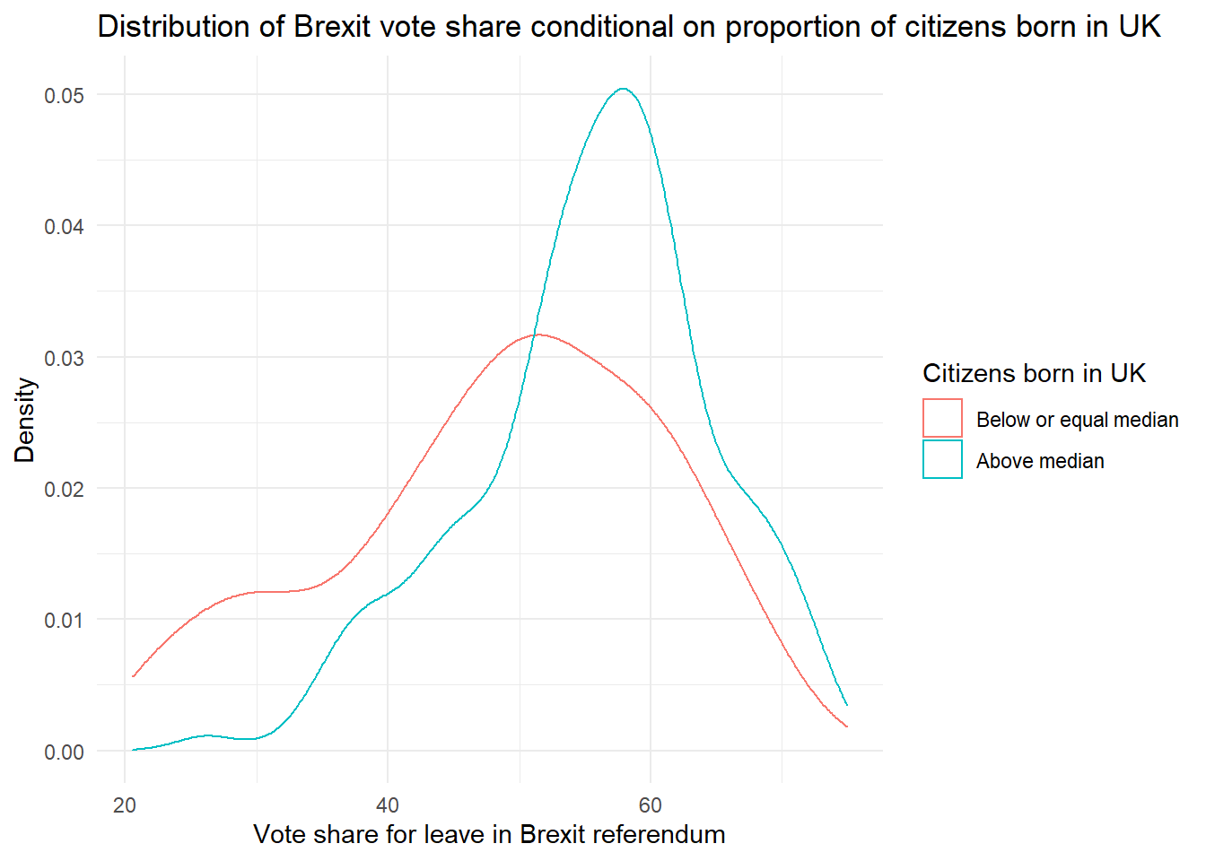

6.2.1.3 Exercise 3

Run a t-test to see if the difference in means statistically significant at an alpha level of 0.05. What about 0.01?

t.test(BrexitVote ~ uk_dummy, 
       data = brexit,
       mu = 0, 
       alt = "two.sided",
       conf = 0.95)


    Welch Two Sample t-test

data:  BrexitVote by uk_dummy
t = -7.9637, df = 576.92, p-value = 8.931e-15
alternative hypothesis: true difference in means is not equal to 0
95 percent confidence interval:
 -8.605085 -5.200260
sample estimates:
mean in group 0 mean in group 1 
       48.62137        55.52405

t.test(BrexitVote ~ uk_dummy, 
       data = brexit,
       mu = 0, 
       alt = "two.sided",
       conf = 0.99)


    Welch Two Sample t-test

data:  BrexitVote by uk_dummy
t = -7.9637, df = 576.92, p-value = 8.931e-15
alternative hypothesis: true difference in means is not equal to 0
99 percent confidence interval:
 -9.142737 -4.662608
sample estimates:
mean in group 0 mean in group 1 
       48.62137        55.52405