3.2 Solutions
Reload the Muslim prejudice data:
# create new outcome variable
table <- mutate(
  table, # call the dataset
  outcome = # new variable called 'outcome'
    case_when(
      is.na(srw_therm_1_h_1) ~ # for those rows where srw_therm_1_h_1 is missing
        srw_therm_2_h_1, # new variable will take value of srw_therm_2_h_1
      is.na(srw_therm_2_h_1) ~ # for those rows where srw_therm_2_h_1 is missing
        srw_therm_1_h_1 # new variable will take value of srw_therm_1_h_1
    )
)3.2.1 Exercise 1
In the Muslim prejudice study, the researchers explain:
Regarding Muslim Americans, media and political actors often promote misperceptions, particularly about Muslims and terrorism… As a result, I evaluated the treatment’s robustness to an environment in which fear of terrorism was present by randomly assigning half of the respondents to a question priming terrorism threats.
This means that this terrorism priming is another treatment variable whose average effect we can estimate through a difference in means. Turn the variable terrorism into a factor variable whose value is “no priming” if it is currently 0 and “primed” if it is currently 1.
We can do this using the factor() function from week 2. It is also possible using mutate() and case_when().
# just using factor()
table$terrorism <- factor(table$terrorism, # specify the variable to make categorical
                          labels = c("no priming", # label corresponding to 0
                                    "primed"), # label corresponding to 1
                          levels = c(0, 1)) # previous levels of variable

# or using mutate() and case_when()
# table <- mutate(table,
#                terrorism = factor(case_when(
#                  terrorism == 0 ~ "no priming",
#                  terrorism == 1 ~ "primed"
#                )))
3.2.2 Exercise 2
Delete all rows with missing values on the outcome variable in your original dataset (called table unless you changed it).
This is easily done with drop_na().
3.2.3 Exercise 3
Visualise the distribution of outcome conditional on terrorism.
A conditional distribution plot, such as the one we made in week 2, works well here:
gg_priming <- ggplot(data = table, # tell R the dataset to work from
                     mapping = aes(x = outcome, # put hdi on the x axis
                                   group = terrorism, # group observations by former colony status
                                   colour = terrorism)) + # allow colour to vary by former colour status
  geom_density() + # create the 'density' geom (the curve, essentially a smoothed histogram)
  labs(x = "Muslim American Feeling Thermometer",
       y = "Density",
       title = "Conditional distribution of feelings towards Muslim Americans",
       subtitle = "Feelings conditional on priming misperceptions about terrorism") + # clearer labels
  theme_minimal() # change the colours

gg_priming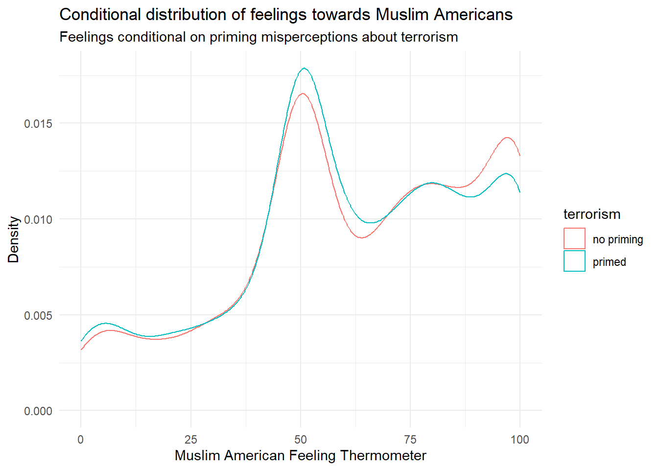
The distributions appear to be very similar, although the most positive feelings seem to be slightly more likely when terrorism misperceptions are not brought to mind.
3.2.4 Exercise 4
Estimate the difference in means, or average treatment effect, of terrorism on the outcome.
# separate two groups
treatment_group <- filter(table, terrorism == "primed")
control_group <- filter(table, terrorism == "no priming")

difference_in_means <-
  mean(treatment_group$outcome) -
  mean(control_group$outcome)

difference_in_means
[1] -1.851343The difference in means is very small, but is in the direction the author expected: those in the control group – whose misperceptions about Muslim involvement in terror attacks were not primed – have a slightly larger mean.
3.2.5 Exercise 5
Estimate the standard error of the difference in means.
We use the formula again:
\[ \sqrt{ \frac{ s^2_{Yx=0} }{ n_{x=0} } + \frac{ s^2_{Yx=1} }{ n_{x=1} }} \]
And apply this in R:
# squared standard deviation in control group
s2ycontrol <- sd(control_group$outcome)^2

# n in control group
ncontrol <- nrow(control_group)

# squared standard deviation in treatment group
s2ytreatment <- sd(treatment_group$outcome)^2

# n in treatment group
ntreatment <- nrow(treatment_group)

# calculation
se_difference_in_means <-
  sqrt( # wrap it all in a square root
    (s2ycontrol/ncontrol) + # control group
      (s2ytreatment/ntreatment) # treatment group
  )

se_difference_in_means
[1] 0.9268306The standard error of the difference in means is approximately 0.93.
3.2.6 Exercise 6
Calculate the 95 percent confidence interval of the difference in means.
[1] -0.03475478[1] -3.667931The confidence interval does not overlap with zero, suggesting that we can reject the null hypothesis at the 95% confidence level.
3.2.7 Exercise 7
Calculate the 99 percent confidence interval of the difference in means. What conclusions can you draw from the result?
[1] 0.5398802[1] -4.242566The confidence interval overlaps with zero, suggesting that we cannot reject the null hypothesis at the 99% confidence level.
3.2.8 Exercise 8
Confirm your results (within errors of rounding) using the t.test() function, first setting conf.level = 0.05 and then conf.level = 0.01.
    Welch Two Sample t-test

data:  outcome by terrorism
t = 1.9975, df = 3577.2, p-value = 0.04585
alternative hypothesis: true difference in means between group no priming and group primed is not equal to 0
95 percent confidence interval:
 0.03417332 3.66851238
sample estimates:
mean in group no priming     mean in group primed
                63.03863                 61.18729
    Welch Two Sample t-test

data:  outcome by terrorism
t = 1.9975, df = 3577.2, p-value = 0.04585
alternative hypothesis: true difference in means between group no priming and group primed is not equal to 0
99 percent confidence interval:
 -0.5372892  4.2399749
sample estimates:
mean in group no priming     mean in group primed
                63.03863                 61.18729