Chapter 10 Going further with the tidyverse: dplyr, magrittr and ggplot2
10.1 dplyr and magrittr
Throughout the early seminars, the code we use frequently shows you a ‘base R’ approach followed by an alternative, so-called ‘tidy’ approach. In nearly every case, these alternatives come from the tidyverse’s popular dplyr package. This package is designed to facilitate clean, easy data management. It is worth having a look through dplyr’s online documentation to understand how this works. Most commonly, we use select(), filter(), and mutate().
10.1.1 The magrittr pipe
These functions become quite powerful when we want to do multiple things to a dataset in one go. Another package from the tidyverse, magrittr, contains a function called the ‘pipe’. The ‘pipe’ operator %>% allows you to write code in a very logical, linear way, in which you start with an object and continually do things to it until you have achieved a desired result.
This becomes clearer with examples. We load a dataset called pop, containing data on the populations of different London boroughs.
#Load a dataset in a csv file
pop <- read.csv("https://raw.githubusercontent.com/QMUL-SPIR/Public_files/master/datasets/census-historic-population-borough.csv")
We might want to subset pop only to contain four variables, but also create a new variable and remove several rows. We could do this all in one ‘pipe’, if we wanted to end up with a new dataset in which all these changes have been made.
# Apply all changes to dataset using pipe

pop_21_200k <- pop %>% # call the dataset
  select( # keep only the variables we want, renaming them
    area_name = Area.Name,
    area_code = Area.Code,
    persons_2001 = Persons.2001,
    persons_2011 = Persons.2011) %>%
  filter( # keep only rows with 200,000+ population
    persons_2011 >= 200000) %>%
  mutate( # create new variable of difference between 2011 and 2001
    persons_diff = persons_2011-persons_2001
  )

# take a look at the new data
head(pop_21_200k)
area_name area_code persons_2001 persons_2011 persons_diff
1 Barnet 00AC 314565 356386 41821
2 Bexley 00AD 218301 231997 13696
3 Brent 00AE 263466 311215 47749
4 Bromley 00AF 295535 309392 13857
5 Camden 00AG 198022 220338 22316
6 Croydon 00AH 330584 363378 32794This code allows you to call the object to which you are applying changes only once. Then, each time you add a function, it takes the object, applies the changes, and passes it through the ‘pipe’ to the next function. So, each function is working on the object churned out by the previous function. Because you are using the pipe, you therefore do not need to specify an object as the first argument of each of these functions. They know automatically what they are working on. This works because in each case, the functions from dplyr (and the rest of the tidyverse) expect a data argument first. The pipe fills this data argument with the result of the previous function. So, in the first case, select() works as follows.
# what we have done in seminars
pop_subset <- select(pop, # name the dataset first as the data argument
                     area_name = Area.Name, # then list the variables we want
                     area_code = Area.Code,
                     persons_2001 = Persons.2001,
                     persons_2011 = Persons.2011)

# pipe alternative
pop_subset <- pop %>% # pass the original dataset into the pipe
  select(area_name = Area.Name, # then just list the variables we want in the function
         area_code = Area.Code,
         persons_2001 = Persons.2001,
         persons_2011 = Persons.2011)
For a single case like this, the piped option isn’t much more efficient, but as above, when we then go on to do several things to the dataset in one go, we gain efficiency. Many people find this approach more intuitive. Consider, for example, that without the pipe, the next stage would be as follows.
# filter newly subsetted dataset as we would have done in class
pop_subset2 <- filter(pop_subset,
                      persons_2011 >= 200000)

# but we could have done this all in one go, without creating new datasets each time
# and without needing to rewrite the dataset name in our code each time
pop_subset2 <- pop %>% # pass the original dataset into the pipe
  select(area_name = Area.Name, # then just list the variables we want in the select function
         area_code = Area.Code,
         persons_2001 = Persons.2001,
         persons_2011 = Persons.2011) %>%
  filter(persons_2011 >= 200000) # then just filter the result
We can try another example of piping on a different dataset. Let’s load the BSAS ‘perceptions of foreigners’ data we have used in previous seminars.
# load perception of non-western foreigners data
load(url("https://github.com/QMUL-SPIR/Public_files/raw/master/datasets/BSAS_manip.RData"))

# look at the first six rows of the dataset
head(data2)
IMMBRIT over.estimate RSex RAge Househld Cons Lab SNP Ukip BNP GP
1 1 0 1 50 2 0 1 0 0 0 0
2 50 1 2 18 3 0 0 0 0 0 0
3 50 1 2 60 1 0 0 0 0 0 0
4 15 1 2 77 2 0 0 0 0 0 0
5 20 1 2 67 1 0 0 0 0 0 0
6 30 1 1 30 4 0 0 0 0 0 0
party.other paper WWWhourspW religious employMonths urban health.good HHInc
1 0 0 1 0 72 4 1 13
2 1 0 4 0 72 4 2 3
3 1 0 1 0 456 3 3 9
4 1 1 2 1 72 1 3 8
5 1 0 1 1 72 3 3 9
6 1 1 14 0 72 1 2 9We want to subset the data only to contain people who overestimated the number of immigrants. We want to assess the proportions of people in this group who identify with each party, which might be easier if we create a single indicator of partisanship rather than having several variables. We also reorganise this data slightly such that the first few columns contain demographic information, followed by our new single indicator of partisanship, followed by the outcome variable IMMBRIT. We don’t think IMMBRIT is a clear enough name, and don’t like how are variable names are formatted inconsistently, so we want to give our variables clearer names and all in snake case.
# create dataset of people who overestimated immigration levels, with reformatting
over_estimators <- data2 %>% # call the original dataframe
  filter( # only keep people who overestimated immigration
    over.estimate == 1
  ) %>%
  mutate( # create single partisanship indicator
    party_id =
      case_when( # function creating variable depending on other variable values
        Cons == 1 ~ "con", # if 'Cons' value is 1, party_id value should be 'con'
        Lab == 1 ~ "lab",
        SNP == 1 ~ "snp",
        Ukip == 1 ~ "ukip",
        BNP == 1 ~ "bnp",
        GP == 1 ~ "green",
        party.other == 1 ~ "other",
        TRUE ~ "none"
        )
  ) %>%
  select( # subset variables (columns)
    sex = RSex,
    age = RAge,
    household = Househld,
    party_id,
    perceived_immigrants = IMMBRIT
  )

# take a look at the new data
head(over_estimators)
sex age household party_id perceived_immigrants
1 2 18 3 other 50
2 2 60 1 other 50
3 2 77 2 other 15
4 2 67 1 other 20
5 1 30 4 other 30
6 2 56 2 snp 60You can see how, if we were only interested in those who overestimate immigration levels, and in certain characteristics of theirs, the over_estimators dataframe would be easier for us to work with. With the %>% pipe, we were able to go from a much larger, less refined dataset, do several clever things to it, and create something more usable and clear, all in one go.
You might be wondering how the case_when() section of this code works. case_when() is a very clever tidyverse function which works like a series of if statements. It is used to create new variables, based on the values of other variables. In each case, it is saying ‘if that variable takes that value, give my the new variable this value’. The ‘if’ statement is expressed before a tilde, ~, with the command (if the statement is true) following the tilde. Finally, TRUE ~ "none" means ‘if none of these things are true, give the new variable the value “none”’. Find out more about case_when() in its documentation.
10.1.2 group_by() and summarise
Further functions from dplyr – namely, group_by() and summarise() – work particularly well with the pipe and highlight its functionality. group_by() groups a dataset by values of a certain variable, so that anything you then do to this dataset will be done separately for each group. summarise() provides a summary of a dataset, in terms set by you. For example, we could group the over_estimators data by party ID. Combining this with summarise, we could then get the average age, and average number of perceived immigrants, within each of these groups.
over_estimators_grpd <- over_estimators %>%
  group_by(party_id) %>%
  summarise(mean_age = mean(age),
            mean_num_imm = mean(perceived_immigrants))

over_estimators_grpd
# A tibble: 7 × 3
party_id mean_age mean_num_imm
<chr> <dbl> <dbl>
1 bnp 38.4 47.4
2 con 54.3 37.0
3 green 49.6 37.7
4 lab 51.8 37.1
5 other 47.3 37.9
6 snp 46.9 35.3
7 ukip 53.2 30.5This would be more complicated to do without the pipe, at least involving creating and storing a new object at each stage. At worst, the code could involve multiple nested functions, which could become very confusing, looking something like this:
over_estimators_grpd <- summarise(group_by(over_estimators, party_id), mean_age = mean(age), mean_num_imm = mean(perceived_immigrants))

over_estimators_grpd
# A tibble: 7 × 3
party_id mean_age mean_num_imm
<chr> <dbl> <dbl>
1 bnp 38.4 47.4
2 con 54.3 37.0
3 green 49.6 37.7
4 lab 51.8 37.1
5 other 47.3 37.9
6 snp 46.9 35.3
7 ukip 53.2 30.5You can imagine how complex such code could become when layering up multiple, more complex pipes, as in the examples above. Nonetheless, the pipe does not allow you to do anything you could not otherwise do in R. There is no requirement for you to learn and use it. However, if you find it useful, it can certainly be a more intuitive and efficient way to write R code.
10.2 ggplot2
Throughout the seminars, we produce plots to visualise distributions of variables and certain relationships of interest. For the most part, we do this using the ggplot() function from the ggplot2 package. This section is included for those who want to understand this better, as well as getting a broader insight into data visualisation. To really get to grips with ggplot2, its online documentation is also extensive and very useful.
10.2.1 Univariate distributions
Sometimes, as you saw in the second seminar, plots are useful to visualise the distribution of a single variable across a dataset. The way in which we do this depends on the level of measurement of the variable.
10.2.1.1 Histograms
The most common way to visualise the distribution of a continuous variable is using histograms. For this example, we use data on Donald Trump’s tweets. It is in .rds format, so we use readRDS() to load it.
# read in the trump datafile
trump_twitter <- readRDS(url("https://github.com/QMUL-SPIR/Public_files/blob/master/datasets/trump_twitter.rds?raw=true"))
You will notice that the data table has 4 columns and 2476 rows. The variables are the text content of the tweet, when it was posted, how many times it was retweeted, and how many times it was favourited.
We could describe this data with simple descriptive statistics, by for example calculating the mean number of times Trump is retweeted, and the standard deviation of this estimate. We could also look at this distribution visually, in the form of a histogram. This can be done very easily in ggplot. Firstly, we can set up the bare bones of the plot.
gg_retweets <- ggplot(data = trump_twitter, # the dataset to work from
                      mapping = aes(x = retweet_count)) # the variables to use
The ggplot(trump, aes(x = retweet_count)) section means create a generic plot object (called gg_retweets) from the trump object using the retweet_count column as the data for the x axis. The data variables are required as ‘aesthetic parameters’ so the retweet_count appears in the aes() brackets. Putting variables within the aes() function essentially allows characteristics of the plot to vary in accordance with these variables. In this case, it is the x axis that varies.
To create the histogram you need to add the relevant geom:
`stat_bin()` using `bins = 30`. Pick better value `binwidth`.
The height of each bar shows the count of the datapoints and the width of each bar is the value range of datapoints included. If you want the bars to be thinner (to represent a narrower range of values and capture some more of the variation in the distribution) you can adjust the binwidth. Binwidth controls the size of ‘bins’ that the data are split up into. Put simply, the bigger the bin (larger binwidth) the more data it can hold. Try:
You can replace the histogram with a smooth density curve. Think of the plotted curve as a summary of the underlying histogram.
gg_trump_dens <- ggplot(data = trump_twitter, # data to work from
                        mapping = aes(x = retweet_count)) +  # axes
  geom_density() # make it a density plot

gg_trump_dens
10.2.1.2 Boxplots
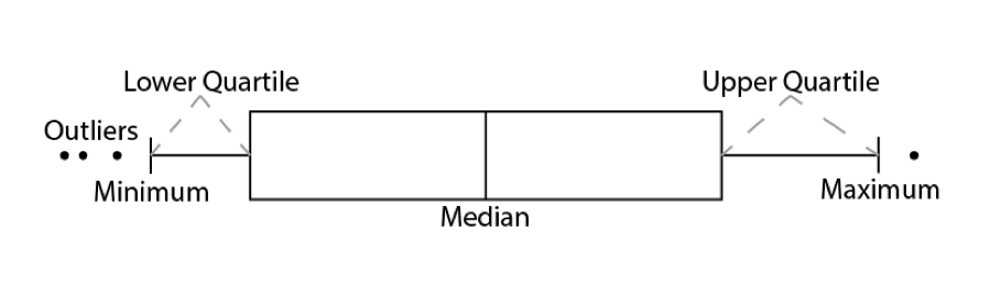
Another common way to visualise distributions of continuous variables, which is sometimes also used for ordinal variables, is using boxplots. Boxplots visualise the median, interquartile range, and full range of a variable. The image below shows how to interpret a boxplot.
The basics remain the same. We tell ggplot() the dataset we want to use, and how to map variables onto the axes, then use a geom to determine the way the data is visualised.
# create boxplot
gg_box <- ggplot(data = trump_twitter, # dataset to work from
                 mapping = aes(x = 1, # any single number fixes the axis
                               y = retweet_count)) + # y axis variable
  geom_boxplot() # make it a boxplot

gg_box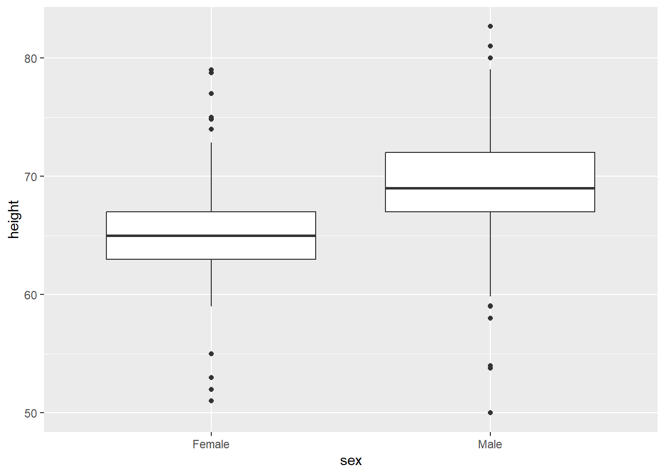
10.2.1.3 Bar charts
For nominal variables, and some types of ordinal variables, visualisation is more limited to simple approaches such as bar plots. For example, we could have a dataset including a marriage status variable. Assume we have 125 unmarried people and 75 married people.
marriage <- data.frame(
  id = 1:200, # unique number for each person
  married = c(rep("married", times = 75), # make first 75 "married"
              rep("unmarried", times = 125)) # make remaining 125 "unmarried"
)

gg_marr <- ggplot(data = marriage, # dataset to work from
                  mapping = aes(x = married)) + # marriage status on x axis
  geom_bar()

gg_marr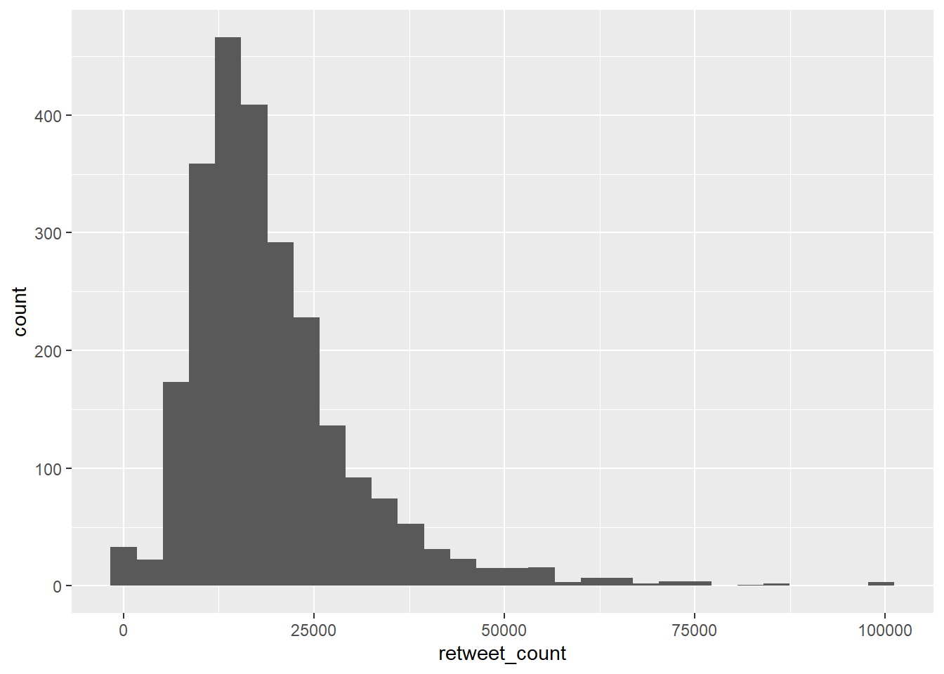
The y axis is automatically set to give us the count of people in the sample who are in each category on the married variable, which we put on the x axis.
10.2.2 Relationships between variables
So far, we have only allowed one variable to affect the visualisation at a time. One of the strengths of data visualisation and its implementation of ggplot2, however, is that it allows you to make multiple visual components vary according to your data. The simplest way to build o what we have done so far is to plot one variable on each axis, visualising the relationship between them.
10.2.2.1 Scatterplots
Perhaps the most common way this is done is in the form of scatterplots. Scatterplots plot two continuous variables against each other. For example, continuing with the Donald Trump Twitter data, we could see whether there is a visible relationship between the number of retweets and the number of favourites (or ‘likes’) he receives. We might sensibly hypothesise that the more retweets he gets, the more likes he is likely to get, because more retweets mean more accounts are exposed to the tweet indirectly.
gg_rt_fav <- ggplot(data = trump_twitter, # dataset to work from
                    mapping = aes(x = retweet_count, # x axis
                                  y = favorite_count)) + # y axis
  geom_point() # make it a scatterplot


gg_rt_fav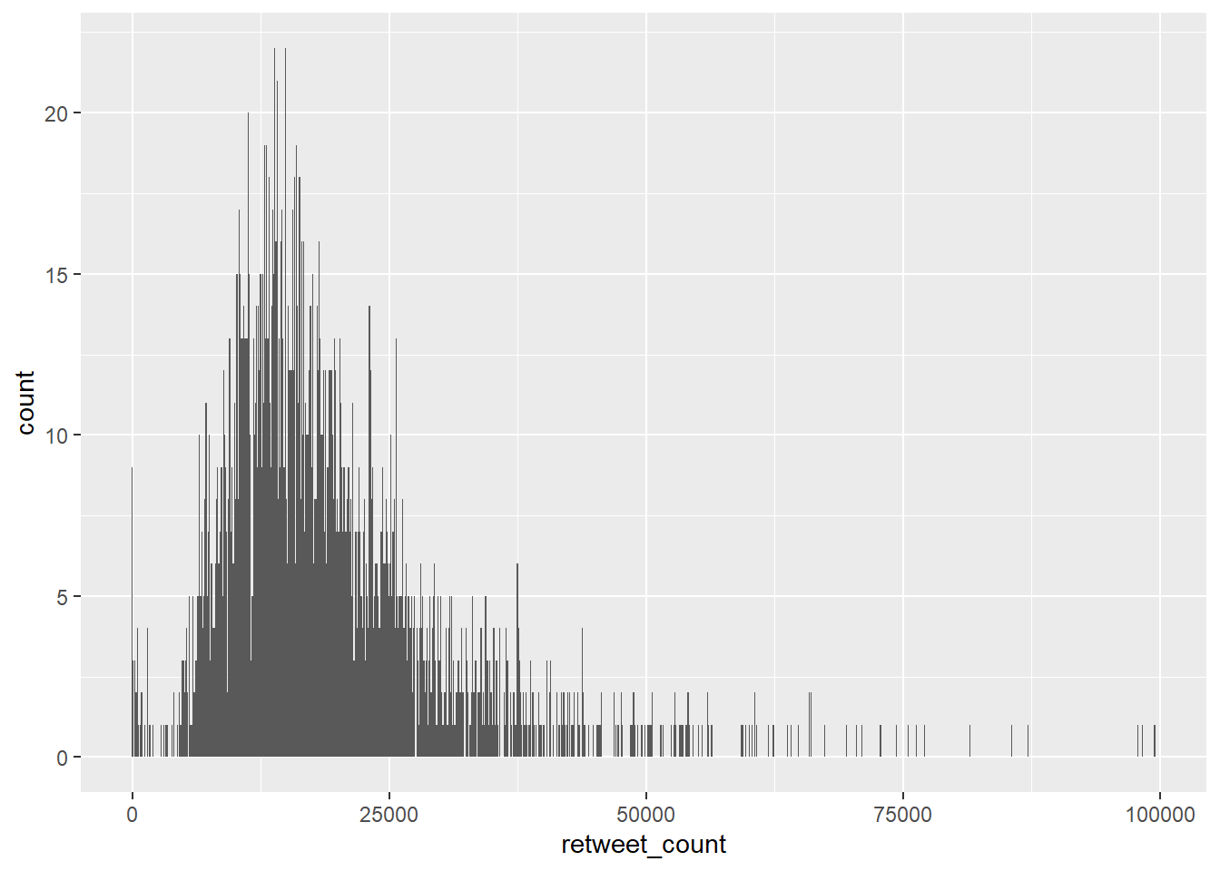
This appears to be correct. There is a clear positive trend. Higher retweets tend to be associated with higher favourite counts.
There are many other ways to visualise relationships. For example, in the second seminar, we used conditional distribution plots to show how a continuous variable’s distribution varied according to a separate categorical variable. We can also use lines, smooths and more complex boxplots.
10.2.3 Increasing complexity
10.2.3.1 Varying aesthetics
In some cases, however, it is difficult to visualise relationships between multiple variables simply using geoms and our axes. Fortunately, it is easy to vary other types of ‘aesthetic’ in ggplot2.
For this example, we use date on transport use in 2020 during the early stages of the coronavirus pandemic.
# download data
mob <- readRDS(url("https://github.com/QMUL-SPIR/Public_files/blob/master/datasets/apple_mobility.rds?raw=true"))

# we will just look at the uk
uk_mob <- filter(mob,
                 region == "United Kingdom")
We can visualise people’s transport use over time as a scatterplot, or a smoothed line.
# scatterplot
gg_tran_scat <- ggplot(data = uk_mob,
                  mapping = aes(x = date,
                                y = score)) +
  geom_point()

gg_tran_scat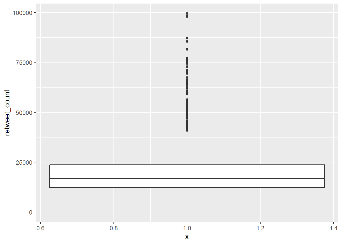
# line
gg_tran_smooth <- ggplot(data = uk_mob,
                  mapping = aes(x = date,
                                y = score)) +
  geom_smooth()

gg_tran_smooth
As we would expect, transport use fell sharply as restrictions were imposed, and then steadily rose again as these were eased. However, this might vary somewhat by the type of transport under consideration. This additional factor can be introduced to the visualisation by varying aesthetics. For example, the colour of the points in the scatterplot can be set to vary by this third variable.
# scatterplot with varying colours
gg_tran_scat <- ggplot(data = uk_mob,
                  mapping = aes(x = date,
                                y = score,
                                colour = transportation_type)) + # vary colour by transport method
  geom_point()

gg_tran_scat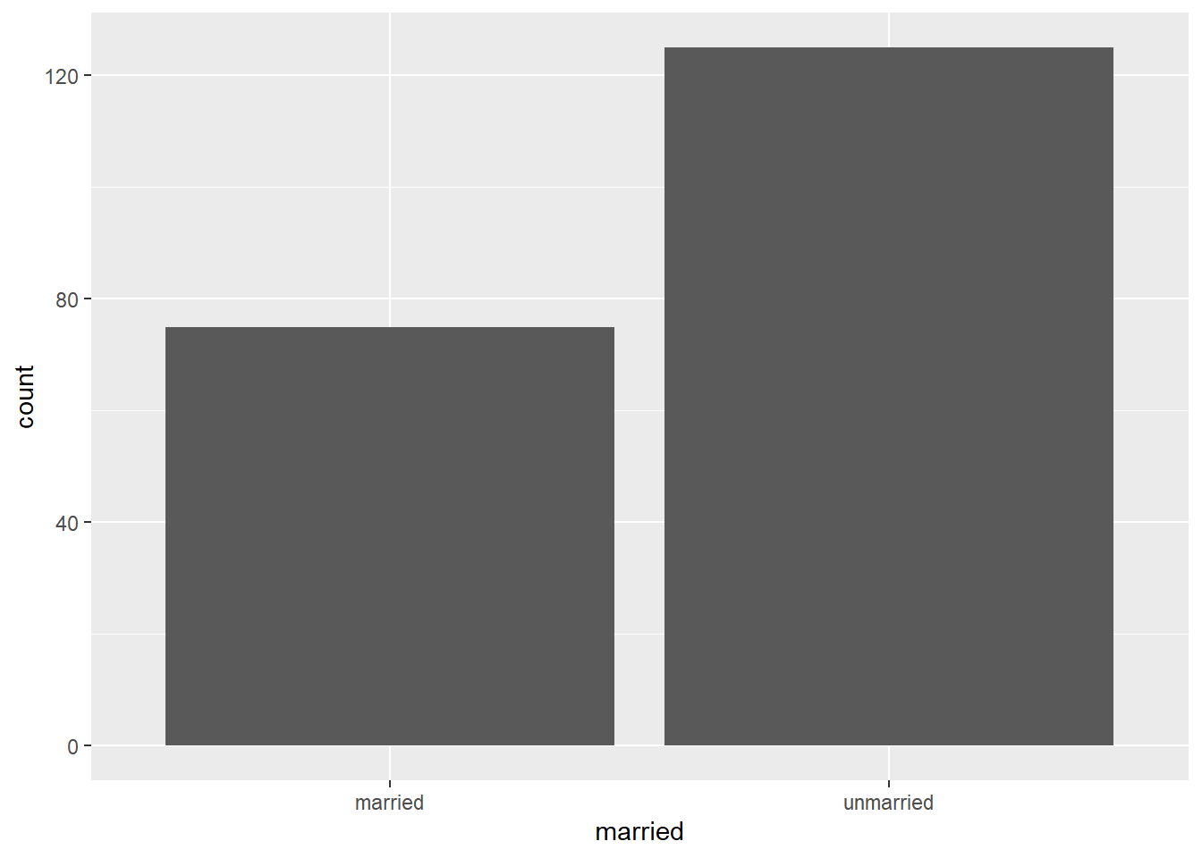
Alternatively, the shapes of the points could vary.
# scatterplot with varying shapes
gg_tran_scat <- ggplot(data = uk_mob,
                  mapping = aes(x = date,
                                y = score,
                                shape = transportation_type)) + # vary colour by transport method
  geom_point()

gg_tran_scat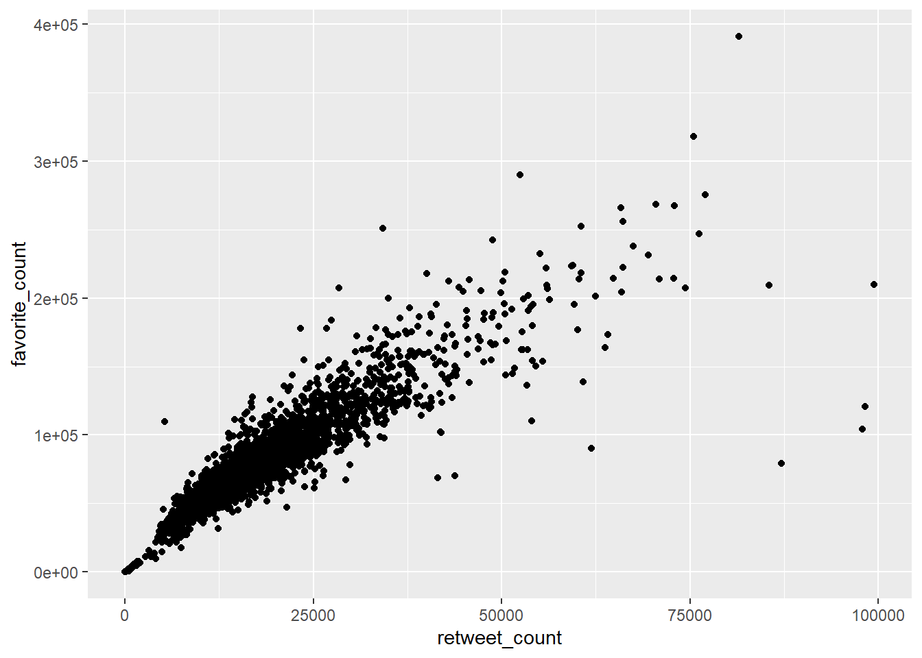
Equally, we could vary the linetype in our smoothed plot.
# smooth with varying linetypes
gg_tran_smooth <- ggplot(data = uk_mob,
                  mapping = aes(x = date,
                                y = score,
                                linetype = transportation_type)) + # vary colour by transport method
  geom_smooth()

gg_tran_smooth
Here again we could vary the colour.
# smooth with varying colours
gg_tran_smooth <- ggplot(data = uk_mob,
                  mapping = aes(x = date,
                                y = score,
                                colour = transportation_type)) + # vary colour by transport method
  geom_smooth()

gg_tran_smooth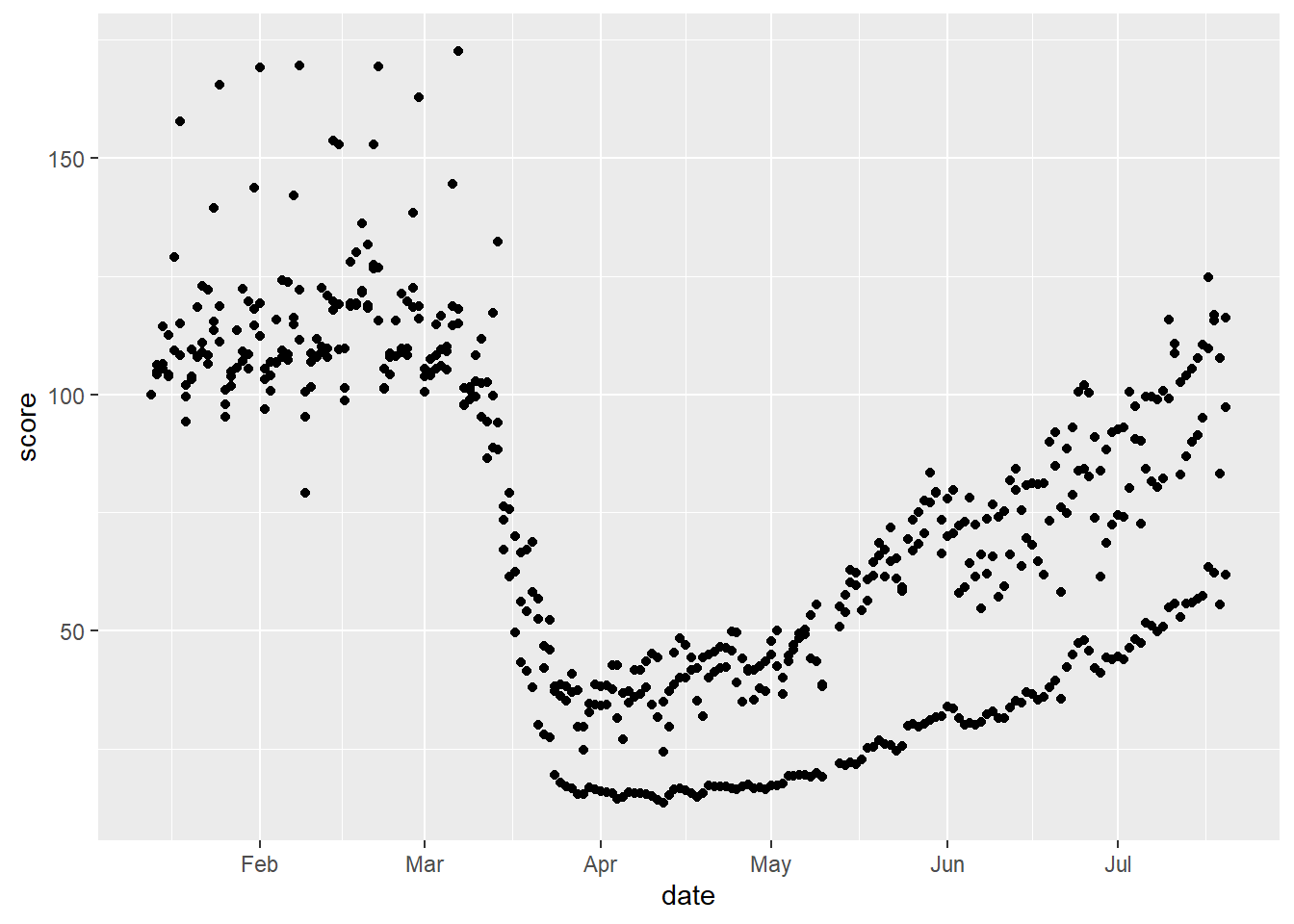
We can even do more than one of these things at once.
# smooth with varying colours and linetype
gg_tran_smooth <- ggplot(data = uk_mob,
                  mapping = aes(x = date,
                                y = score,
                                linetype = transportation_type, # vary linetype by transport method
                                colour = transportation_type)) + # vary colour by transport method
  geom_smooth()

gg_tran_smooth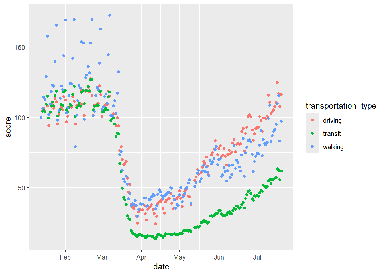
# scatterplot with varying colours and shapes
gg_tran_scat <- ggplot(data = uk_mob,
                  mapping = aes(x = date,
                                y = score,
                                shape = transportation_type, # vary linetype by transport method
                                colour = transportation_type)) + # vary colour by transport method
  geom_point()

gg_tran_scat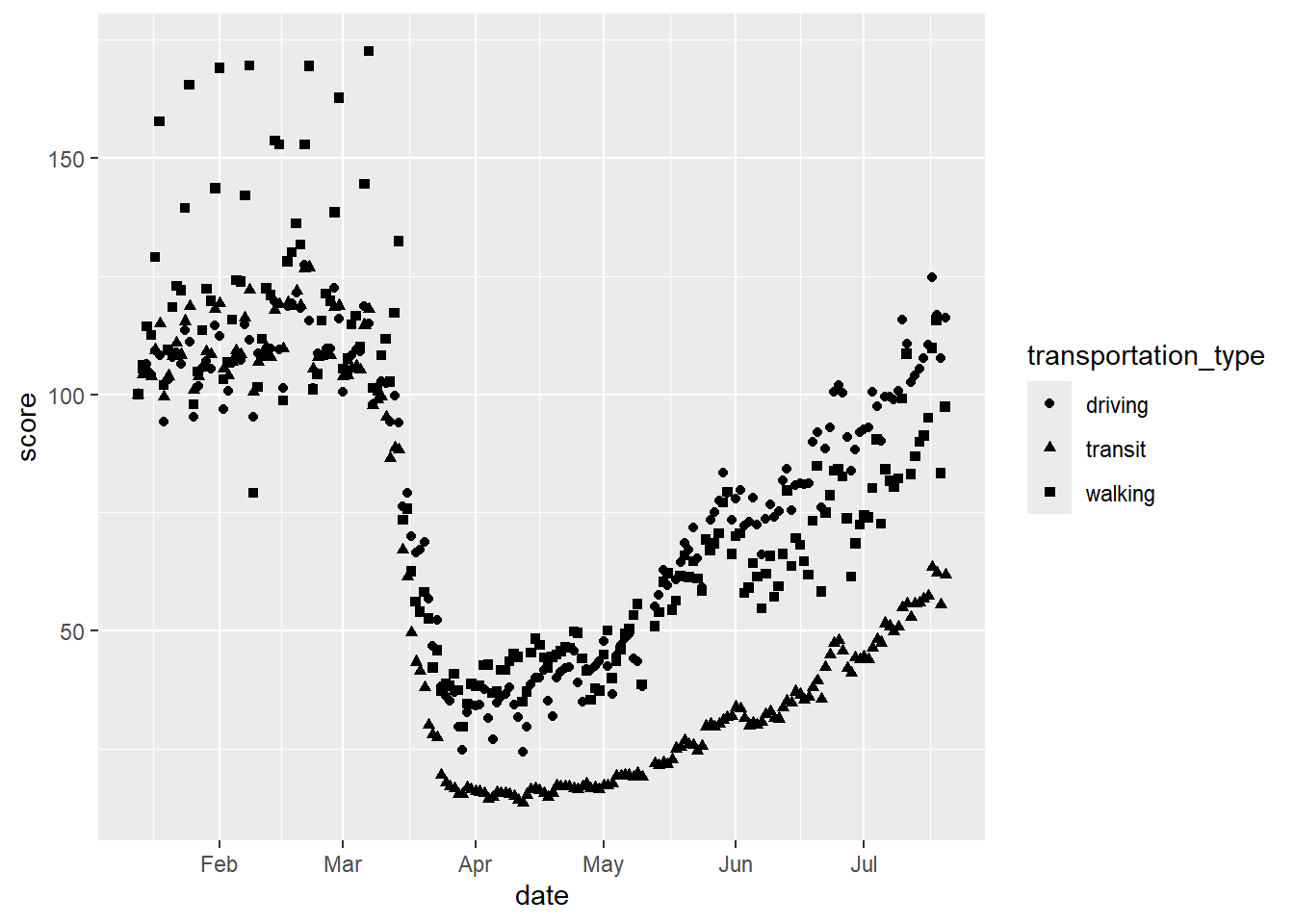
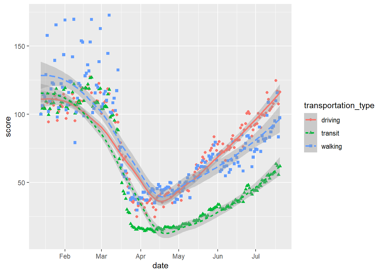
And even combine both geoms with all of these varying aesthetics:
# scatter and smooth with varying colours, linetype and shapes
gg_tran_smooth_scat <- ggplot(data = uk_mob,
                              mapping = aes(x = date,
                                            y = score,
                                            shape = transportation_type, # vary point shape by transport method
                                            linetype = transportation_type, # vary linetype by transport method
                                            colour = transportation_type)) + # vary colour by transport method
  geom_point() + geom_smooth()

gg_tran_smooth_scat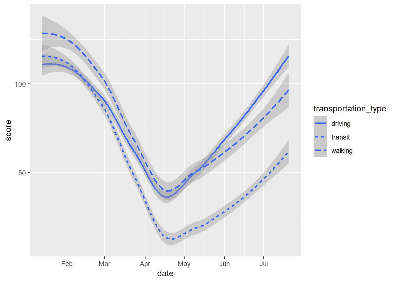
10.2.3.2 Facets
In other cases, it will be easier to use ‘facets’ to split a single plot into multiple subsets, in order to show differences by some additional variable.
Take the following simple example. The heights object contains the reported heights of a group of students.
# read in the heights datafile

heights <- readRDS(url("https://github.com/QMUL-SPIR/Public_files/blob/master/datasets/heights.rds?raw=true"))
We can plot this as a histogram:
# histogram

gg_height <- ggplot(data = heights,
                    mapping = aes(x = height)) +
  geom_histogram()

gg_height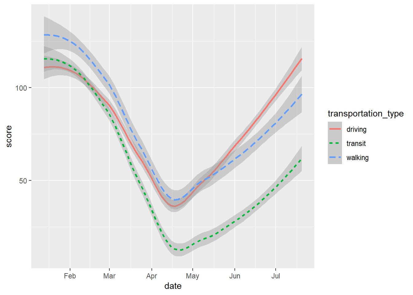
We could also plot this as a boxplot:
# boxplot

gg_height_box <- ggplot(data = heights,
                        mapping = aes(x = 1, y = height)) +
  geom_boxplot()

gg_height_box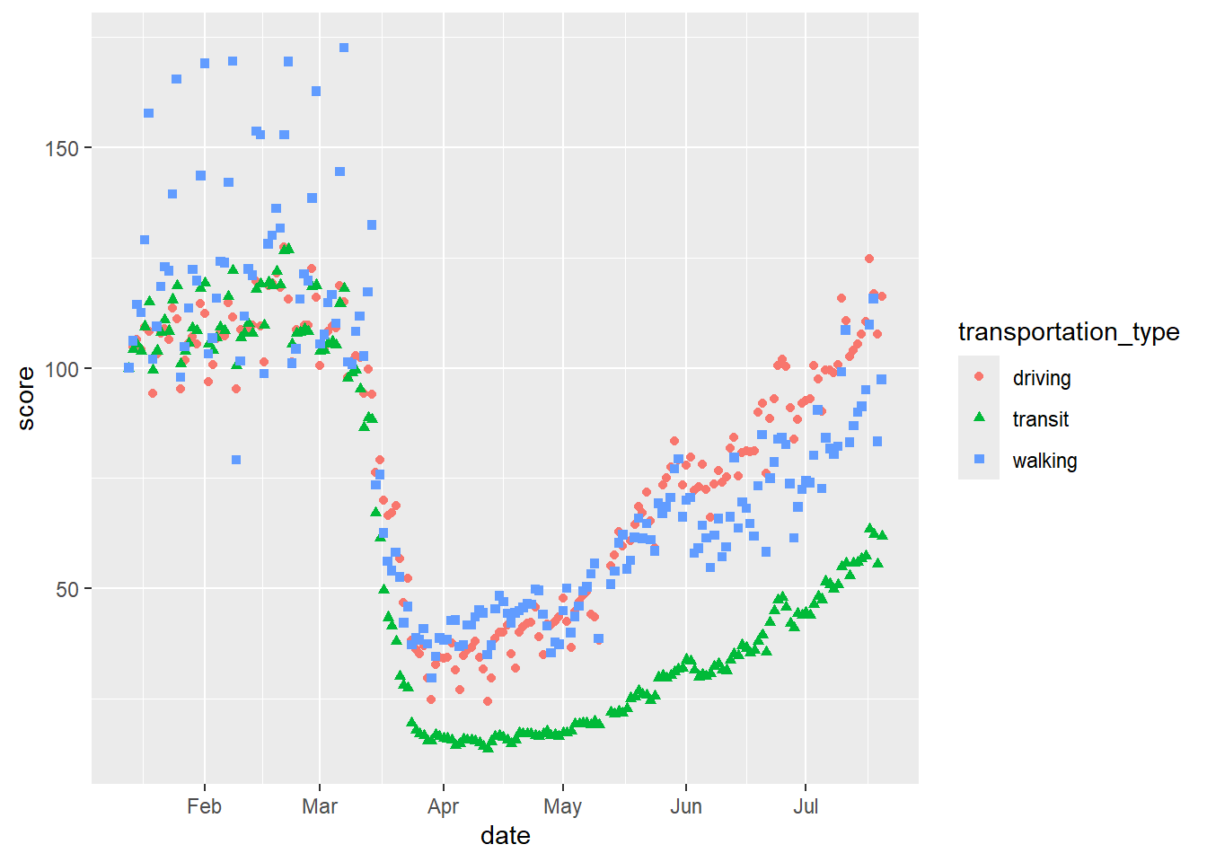
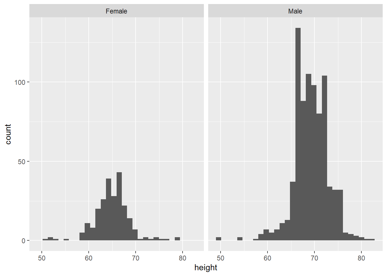
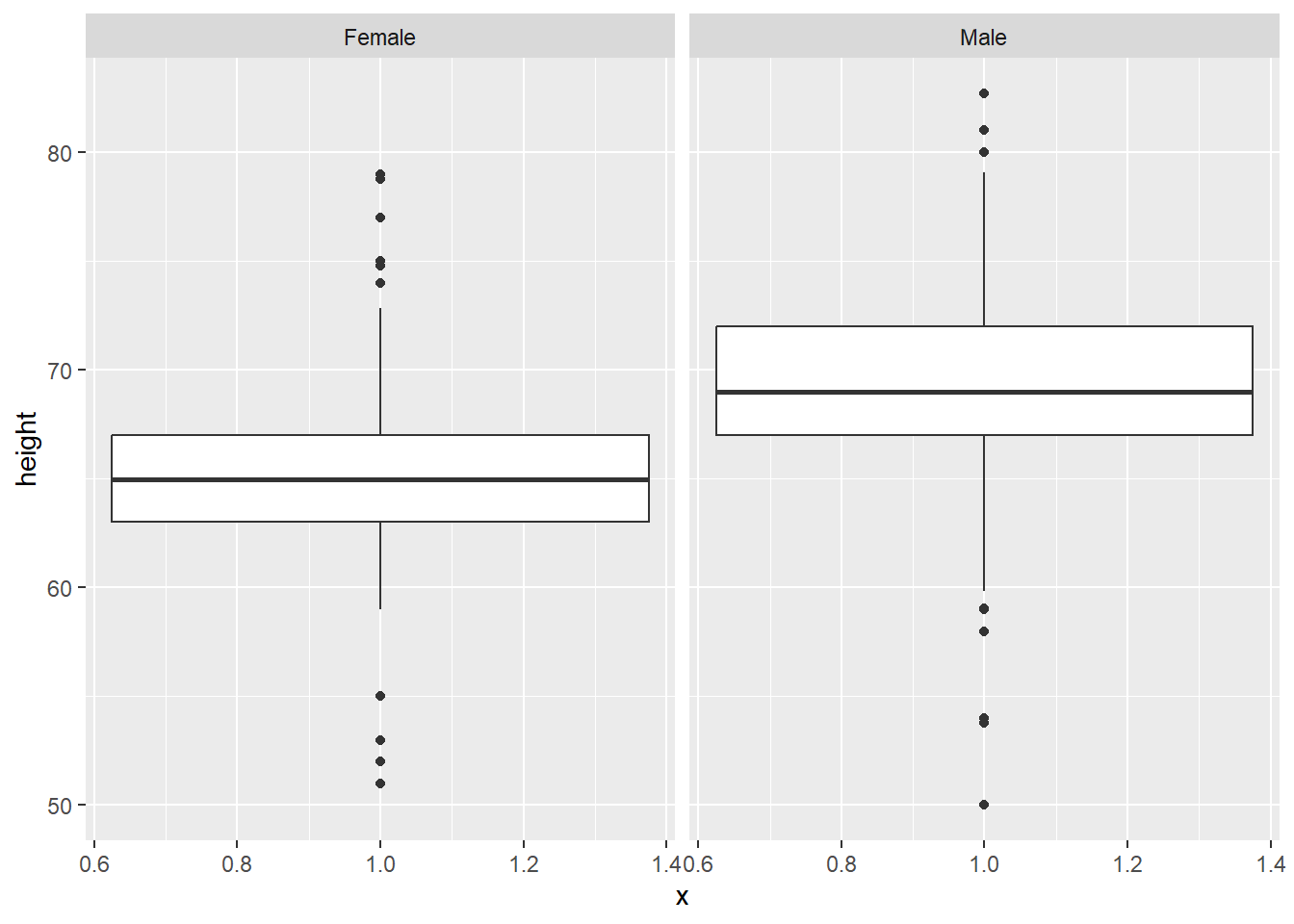
However, we also have data on the students’ reported sex. We know that, on average, men tend to be taller than women. So, we can look at their heights separately using facet_wrap, which splits the plot into different ‘facets’:
The variable after the ‘tilde’ (~) is used to create the different ‘facets’ or panes. This reveals, indeed, that male students are more clustered around taller heights, while female students tend to be less tall on average. This also shows us that we seem to have far more male students in the dataset.
We can do the same thing with virtually any plot, as long as we have a variable to facet by. This also works for boxplots:
But also, with boxplots, it might be clearer to compare within the same plot, by setting sex as the x axis variable:
# boxplot comparison

gg_height_box <- ggplot(data = heights, aes(x = sex, y = height)) +
  geom_boxplot()

gg_height_box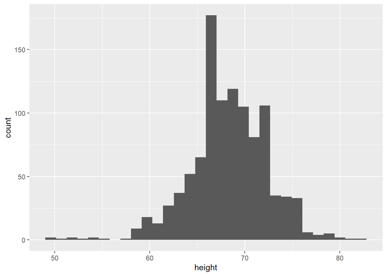
10.2.4 Presentation
Beyond these technical points, it is also important to present plots clearly. You might even want your plots to be visually appealing, as well as easy to understand. The flexibility of ggplot2 means you can change almost everything you see in the plots you create, simply by adding more layers to the code. We will focus here on labels, legends and themes.
10.2.4.1 Labels
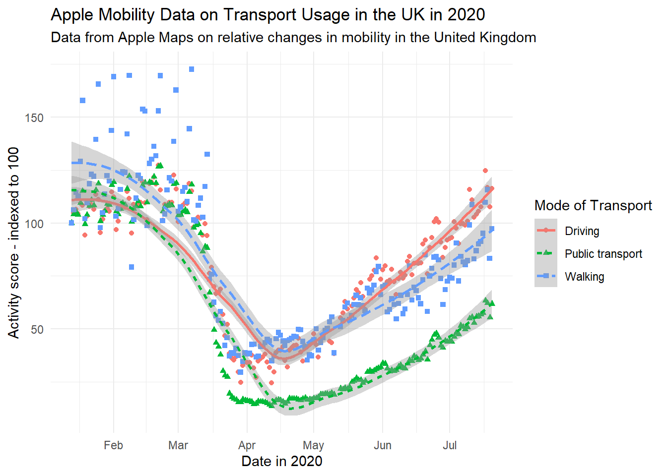
By labels, we refer to the text around the plot designed to explain what it refers to. This includes an overall title (and sometimes subtitle), the axis titles and labels for specific values on the axes. The plots above, for the most part, have labels that are unclear or otherwise not formatted in a presentable, appealing way. Take for example gg_tran_smooth_scat. There is no title or subtitle, and the axis labels are not capitalised. Moreover, ‘score’ does not clearly explain what exactly the y axis refers to. There are several ways to change these labels, but the labs() function is perhaps the simplest, catch-all approach:
gg_tran_smooth_scat <- gg_tran_smooth_scat +
  labs(x = "Date in 2020", # clarify the x axis interpretation
       y = "Activity score - indexed to 100", # clearer y axis
       title = "Apple Mobility Data on Transport Usage in the UK in 2020", # clear, succinct title
       subtitle = "Data from Apple Maps on relative changes in mobility in the United Kingdom") # more explanatory subtitle

gg_tran_smooth_scat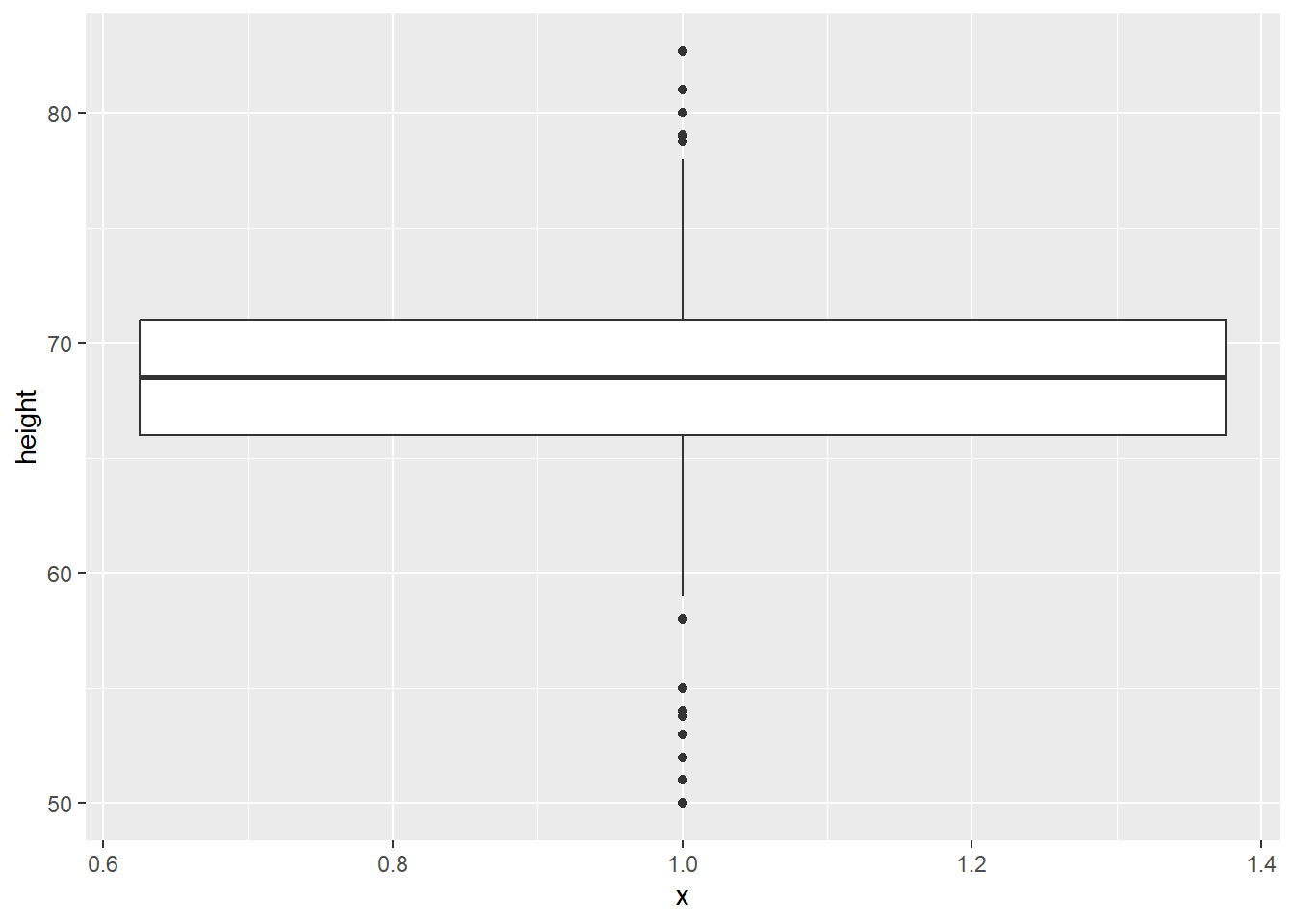
It is now clear to anyone viewing this plot what it shows and how its axes should be interpreted.
10.2.4.2 Legends
When using aesthetic mappings, it is also important to make sure the interpretation of these is clear. This is done by the ‘legend’, which you might also have heard referred to as a ‘key’. In this example, note that even now our plot is labelled clearly, the legend is still not presented properly. Its title, transportation_type, is drawn directly from the column name in the dataset, there is no capitalisation, and ‘transit’ is not a commonly used term in British English. We can overwrite all these things using scale functions. When using multiple aesthetic mappings, as we are here, this needs to be done individually for each one, to keep them together on one consistent legend.
gg_tran_smooth_scat <- gg_tran_smooth_scat +
  scale_colour_discrete( # overwrite colour legend
    name = "Mode of Transport", # change legend title
    labels = c( # change legend labels
      "Driving",
      "Public transport",
      "Walking"
    )
  ) +
  scale_shape_discrete( # overwrite shape legend
    name = "Mode of Transport", # change legend title
    labels = c( # change legend labels
      "Driving",
      "Public transport",
      "Walking"
    )
  ) +
  scale_linetype_discrete( # overwrite shape legend
    name = "Mode of Transport", # change legend title
    labels = c( # change legend labels
      "Driving",
      "Public transport",
      "Walking"
    )
  )

gg_tran_smooth_scat
The meanings of the different colours, shapes and linetypes are now completely clear to anyone viewing this plot.
10.2.4.3 Themes
By default, ggplot2 creates plots with a grey grid in the background, and making certain assumptions about what text you want included. This is the default ‘theme’. This can be changed using theme_ functions. Many people simply do not like the appearance of the grey background, so change the theme for that reason, but theme() also allows you to change much more – including, indeed, the labels and legend.


# edit label appearance
gg_tran_smooth_scat +
  theme(axis.title = element_text(size = 14), # large axis labels
        axis.text = element_text(colour = "blue"), # blue axis text
        plot.title = element_text(size = 16, colour = "blue"), # large blue title
        plot.subtitle = element_text(face = "italic")) # italicised subtitle
# edit legend appearance
gg_tran_smooth_scat +
  theme(legend.background = element_rect(fill = "grey"), # give the legend a grey background
        legend.title = element_text(size = 14), # larger legend title
        legend.text = element_text(face = "italic")) # italicised legend labels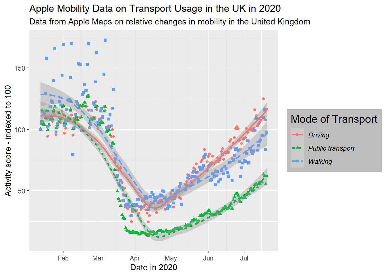
These are just a few examples of changes that are mostly superficial, but they can sometimes become very useful in easing the interpretation of your data visualisations. Note that you can essentially layer as many of these changes as you like, for fully personalised plots.
10.2.5 Example – data visualisation in practice
We have a dataset about penguins:
# read in the penguins datafile

penguins <- readRDS(url("https://github.com/QMUL-SPIR/Public_files/blob/master/datasets/penguins.rds?raw=true"))
We can visualise the distribution of a single variable, for example flipper length, using a histogram.
flipper_hist <- ggplot(data = penguins,
                       mapping = aes(x = flipper_length_mm)) +
  geom_histogram()

flipper_hist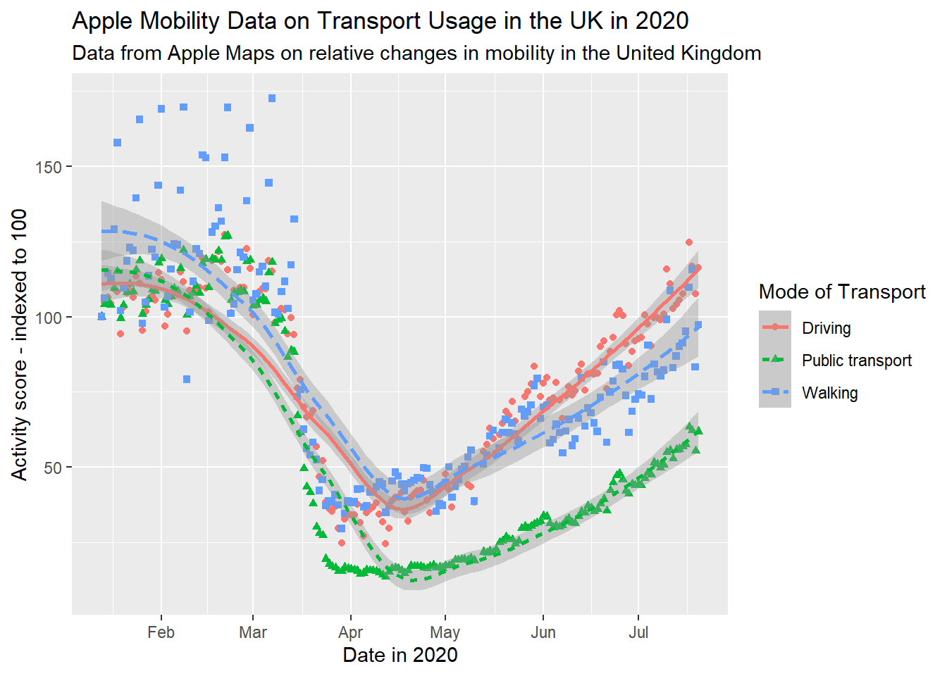
However, we know that different species of penguins come in different sizes. So we can take the histogram and add a facet_wrap layer to see this.
We might be interested in visualising the relationship between different penguin characteristics. For example, we could create a scatterplot to show the relationship between bill depth and bill length.
bill_scatter <- ggplot(data = penguins,
                       mapping = aes(x = bill_depth_mm, y = bill_length_mm)) +
  geom_point() +
  geom_smooth(method = "lm") # add this to see the direction of the linear relationsip

bill_scatter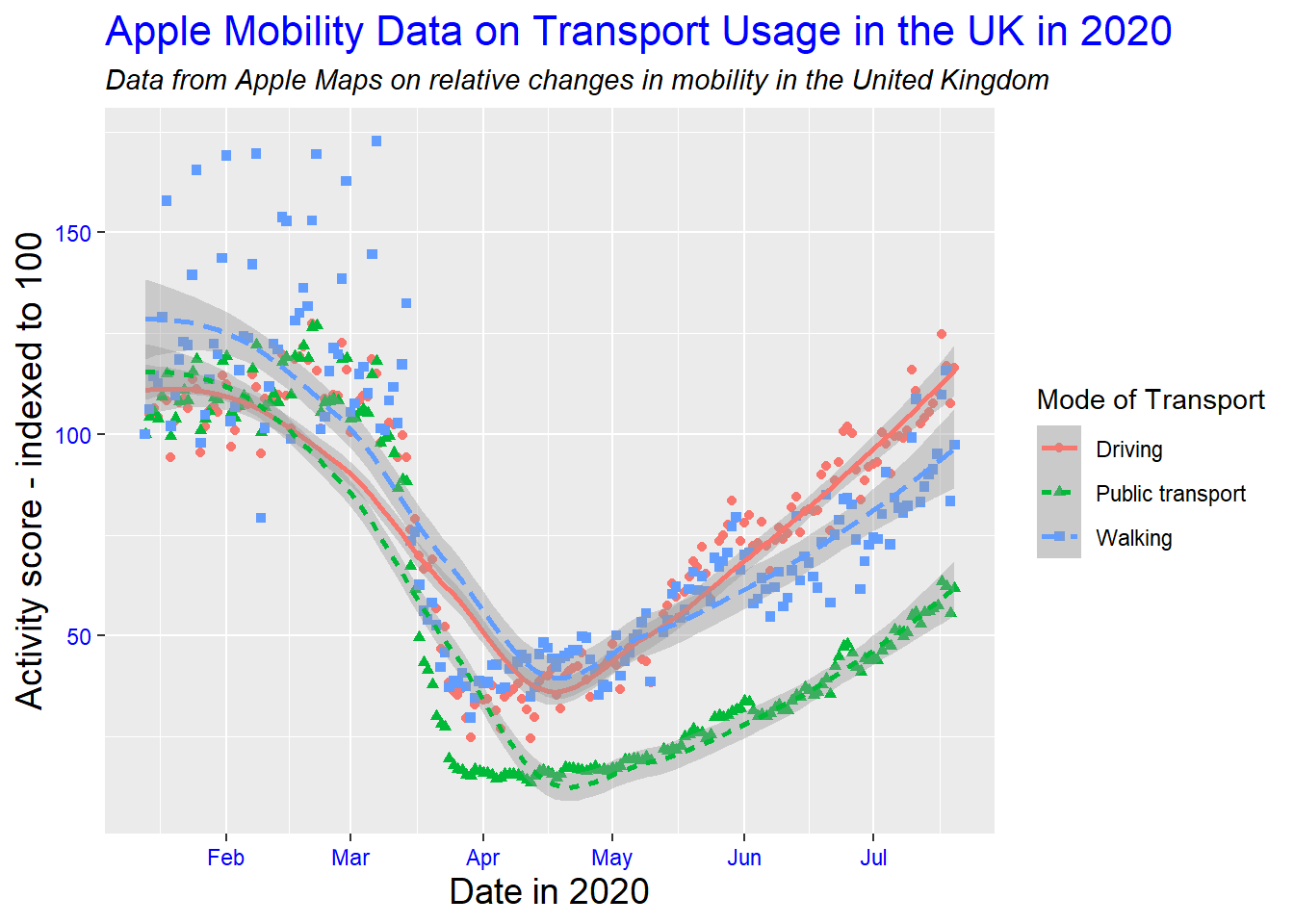
There appears to be a weak negative relationship between bill depth and bill length – deeper bills tend to be shorter in length. Is this what we would expect? It seems strange that beaks that are bigger in one sense would tend to be smaller in another sense. It is hard to imagine penguins with very long but thin beaks, for example.
We know, however, from what we saw above, that different species come in different sizes and this is related to the size of their body parts. How does this beak relationship change when we break it down into species?
bill_scatter_species <- ggplot(data = penguins,
                               mapping = aes(x = bill_depth_mm,
                                             y = bill_length_mm,
                                             colour = species,
                                             shape = species)) +
  geom_point() +
  geom_smooth(method = "lm")

bill_scatter_species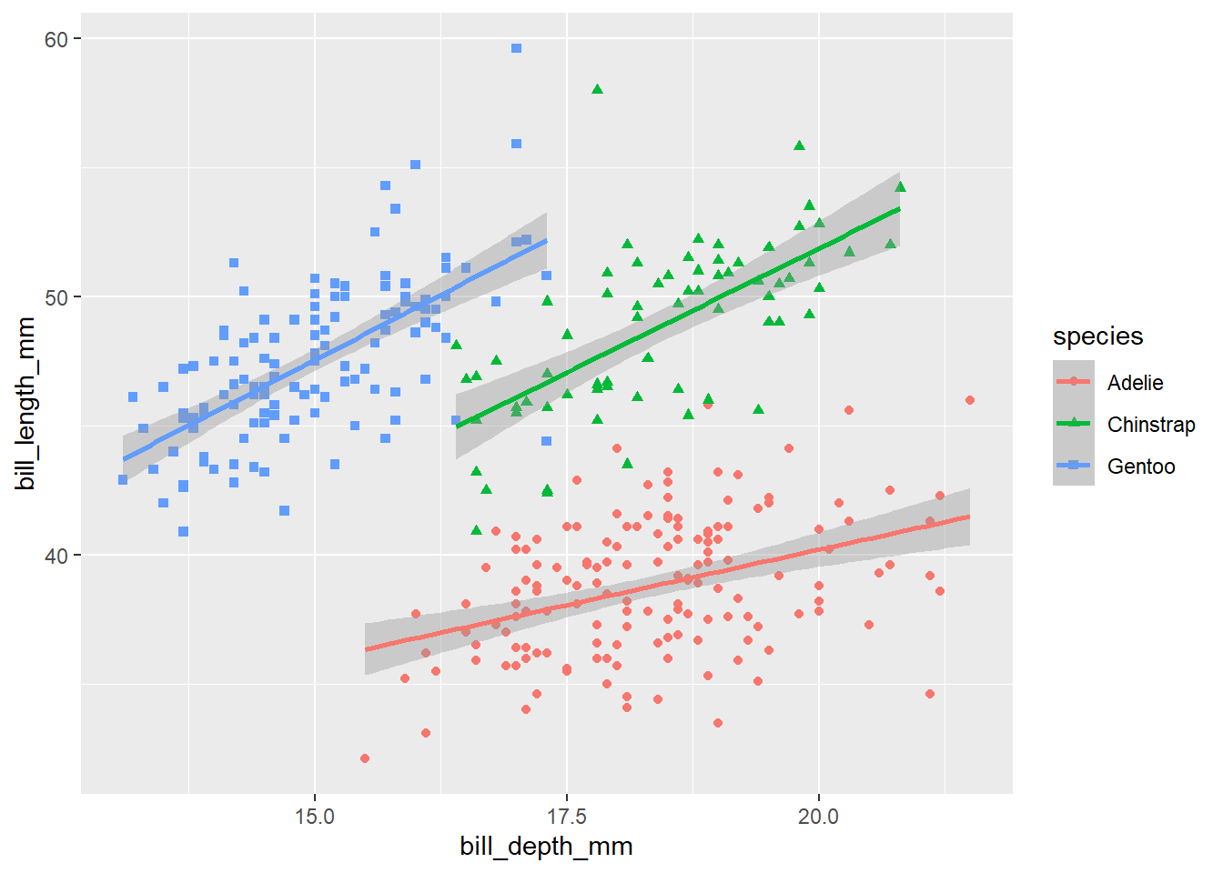
Now, we can tidy up this plot to make it clearer.
bill_scatter_species <- bill_scatter_species +
  labs(title = "Relationship between penguin bill depth and length, by species",
       subtitle = "For a given species, deeper bills tend to be longer",
       x = "Bill depth (mm)",
       y = "Bill length (mm)") +
  scale_colour_discrete(name = "Species of penguin") +
  scale_shape_discrete(name = "Species of penguin") +
  theme_classic() +
  theme(plot.subtitle = element_text(face = "italic"))

bill_scatter_species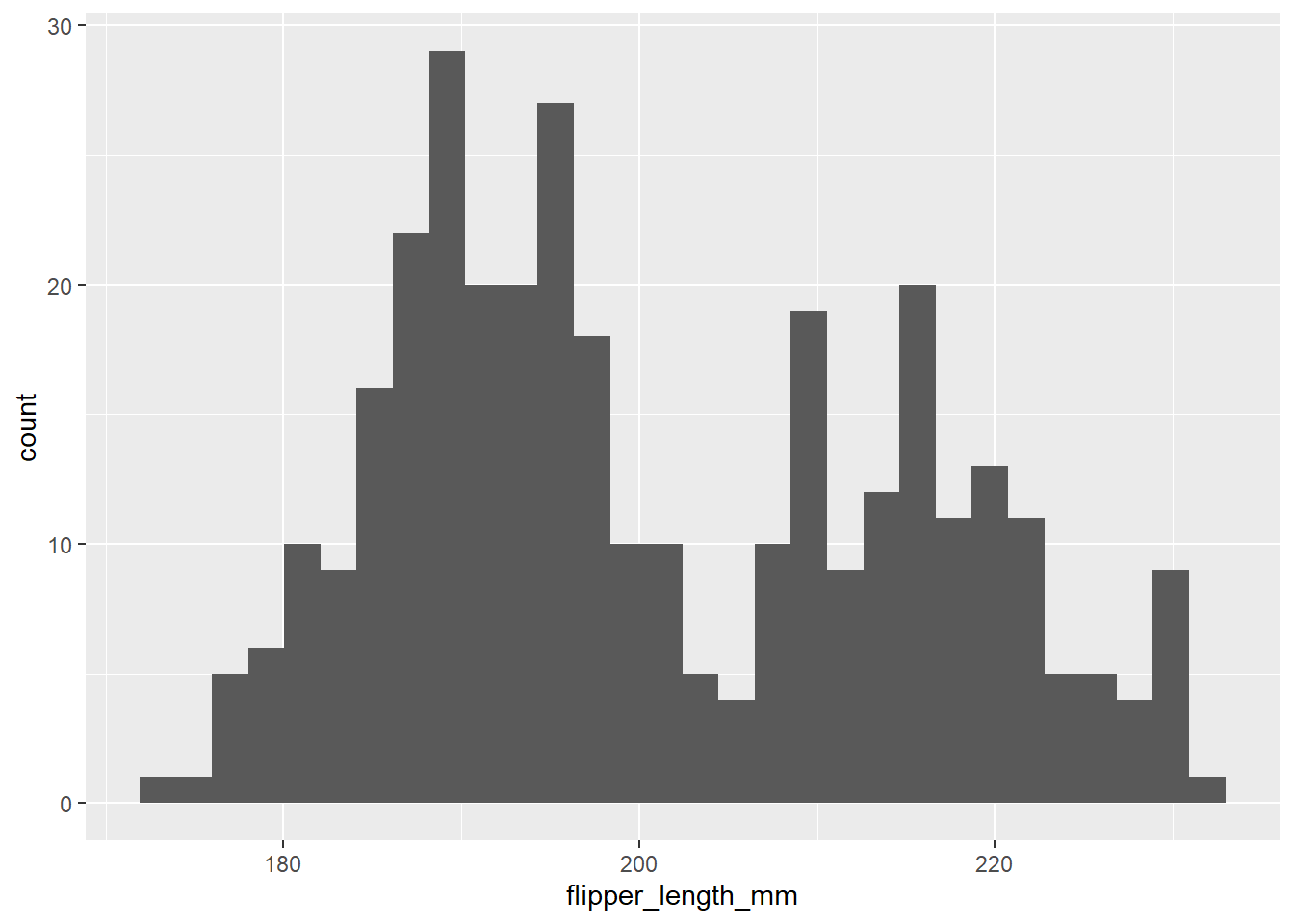
Now, we can see very clearly that, within each species of penguin, there is a positive relationship between bill depth and length. This relationship is masked by the fact that different species of penguin have different sized bills overall. What we have uncovered here, through data visualisation, is an example of Simpson’s paradox. This paradox occurs when a relationship within groups disappears or reverses when those groups are aggregated together, as here. Data visualisation helps us to explore and understand relationships like this in our data – and, importantly, to present them clearly.
10.2.6 Combining dplyr, magrittr and ggplot2
Note that, while ggplot2 does not use piped code, it is possible to integrate a ggplot2 call to the end of a magrittr pipe, which also includes dplyr functions. For example, suppose we wanted to plot the mean and 95% confidence interval for each penguin species’ bill length, as a dot and whisker or ‘pointrange’ plot. We could use piped dplyr code to estimate to estimate those things, then add a ggplot2 call to the end of the pipe to plot the results. As this is piped, we do not need to fill the data argument in the ggplot() function.
In this code, we estimate the confidence intervals manually, by first getting the standard error (standard deviation divided by the square root of the sample size), multiplying this by 1.96 and adding/subtracting it from the mean.
grpd_pngn_plot <- penguins %>% # call the dataset
  drop_na(bill_length_mm) %>% # first we remove any missing values on the bill_length_mm variable
  group_by( # group into different species
    species) %>%
  summarise( # estimate group means and CIs
    mean = mean(bill_length_mm), # group means
    upper_ci = mean(bill_length_mm) + 1.96*(sd(bill_length_mm)/sqrt(length(bill_length_mm))), # group confidence interval bounds
    lower_ci = mean(bill_length_mm) - 1.96*(sd(bill_length_mm)/sqrt(length(bill_length_mm)))
  ) %>%
  ggplot(mapping = aes(x = species,
                       y = mean,
                       ymin = lower_ci,
                       ymax = upper_ci)) +
  geom_pointrange() +
  labs(x = "Species of Penguin",
       y = "Mean and 95% confidence intervals of bill length (mm)") +
  theme_minimal()

grpd_pngn_plot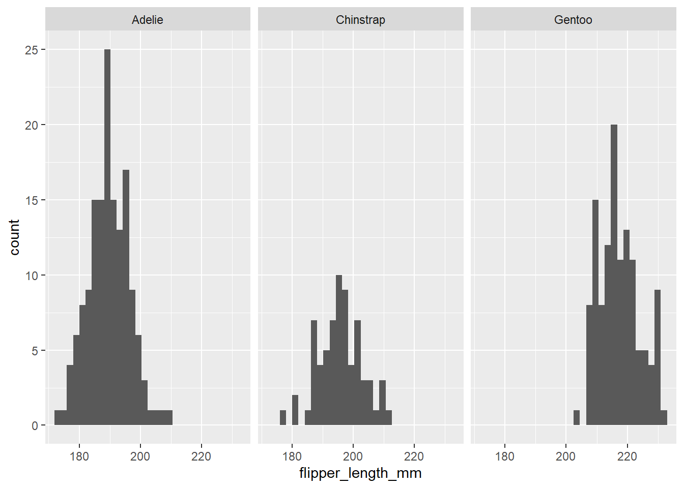
This, indeed, confirms that we can be quite confident that different species of penguins’ bills differ systematically in length!