Chapter 1 Introduction: Measurement, Central Tendency, Dispersion
1.1 Seminar – in class exercises
In this seminar session, we introduce working with R. We illustrate some basic functionality and help you familiarise yourself with the look and feel of RStudio. Measures of central tendency and dispersion are easy to calculate in R. We focus on introducing the logic of R first and then describe how central tendency and dispersion are calculated in the end of the seminar.
1.1.1 Getting Started
You should have already installed R and RStudio. If you haven’t, install them on your computer by downloading them from the following sources:
- Download R from The Comprehensive R Archive Network (CRAN)
- Download RStudio from RStudio.com
1.1.2 RStudio
We use R through RStudio. R is just a statistical programming language, and RStudio provides a user-friendly interface to interact with this language. When you start RStudio for the first time, you’ll see three panes:
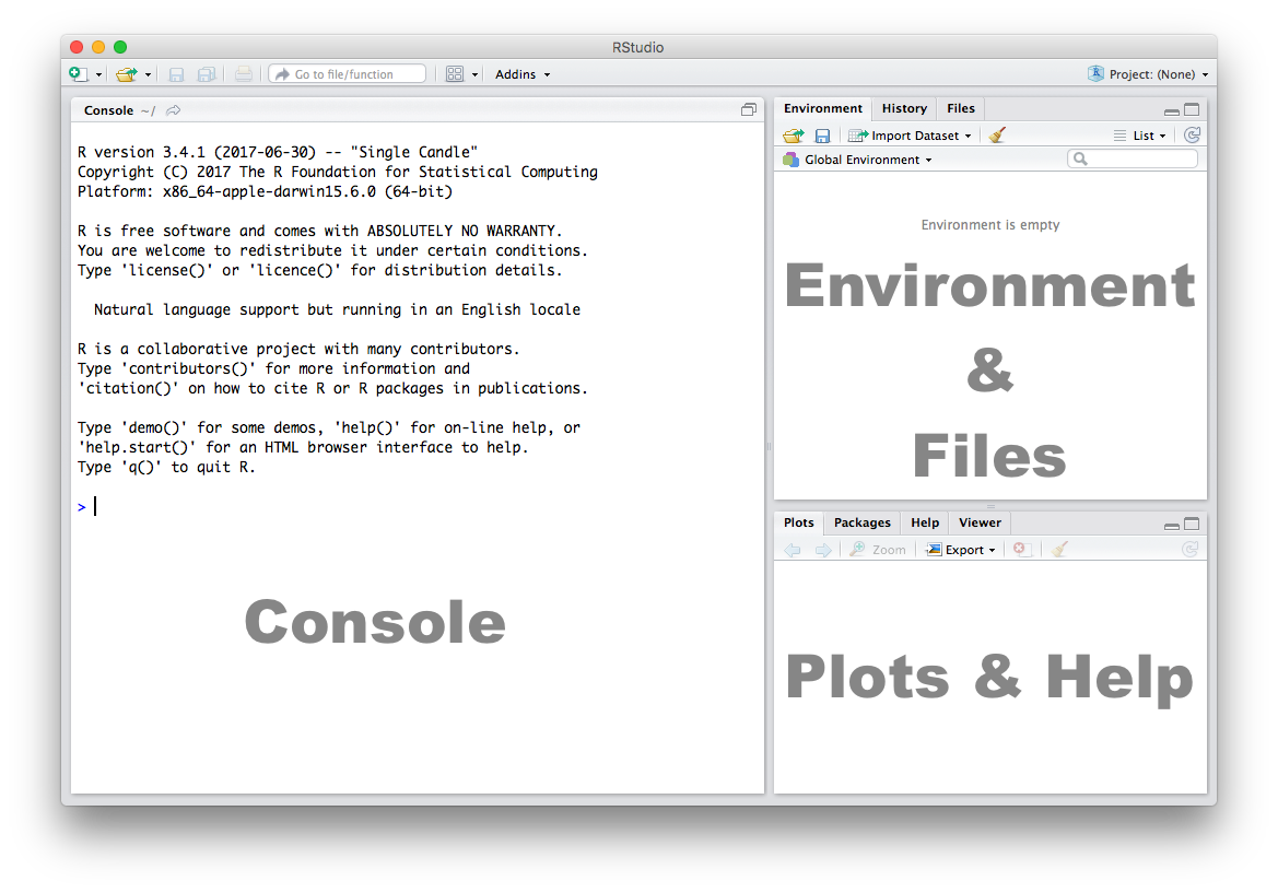
1.1.2.1 Console
The Console in RStudio is the simplest way to interact with R. You can type some code at the Console and when you press ENTER, R will run that code. Depending on what you type, you may see some output in the Console or if you make a mistake, you may get a warning or an error message.
Let’s familiarize ourselves with the console by using R as a simple calculator:
[1] 6Now that we know how to use the + sign for addition, let’s try some other mathematical operations such as subtraction (-), multiplication (*), and division (/).
[1] 6[1] 15[1] 3.5| You can use the cursor or arrow keys on your keyboard to edit your code at the console: - Use the UP and DOWN keys to re-run something without typing it again - Use the LEFT and RIGHT keys to edit |
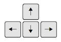 |
Take a few minutes to play around at the console and try different things out. Don’t worry if you make a mistake, you can’t break anything easily!
1.1.2.2 Functions
Functions are a set of instructions that carry out a specific task. Functions often require some input and generate some output. For example, instead of using the + operator for addition, we can use the sum function to add two or more numbers.
[1] 15In the example above, 1, 4, 10 are the inputs and 15 is the output. A function always requires the use of parenthesis or round brackets (). Inputs to the function are called arguments and go inside the brackets. The output of a function is displayed on the screen but we can also have the option of saving the result of the output. More on this later.
1.1.2.3 Getting Help
Another useful function in R is help which we can use to display online documentation. For example, if we wanted to know how to use the sum function, we could type help(sum) and look at the online documentation.
The question mark ? can also be used as a shortcut to access online help.
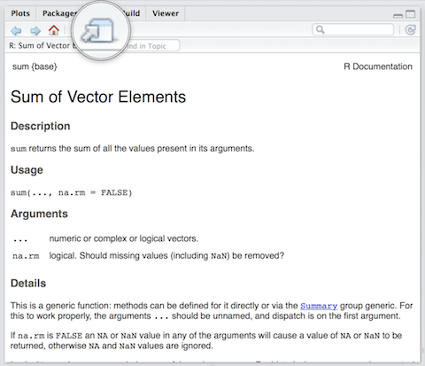
Use the toolbar button shown in the picture above to expand and display the help in a new window.
Help pages for functions in R follow a consistent layout generally include these sections:
| Description | A brief description of the function |
| Usage | The complete syntax or grammar including all arguments (inputs) |
| Arguments | Explanation of each argument |
| Details | Any relevant details about the function and its arguments |
| Value | The output value of the function |
| Examples | Example of how to use the function |
1.1.2.4 Packages – the tidyverse
R comes with some core functionality and allows users to add to this. These add-ons are called packages. We first need to install a package (but only once). Every time we start R, we need to load the package.
To install a package, we write install.packages("packagename"). To load a package, we write library(packagename).
Throughout this and future seminars, we will usually show you standard ways to do things using R’s ‘base’ functionality, but in many cases there are different (more ‘tidy’) ways to do things that some people find more intuitive, using other packages. We will aim to show you these alternative approaches too, where relevant. They tend to use functions from the ‘tidyverse’, which you will need to install and load. This can be done easily from within RStudio:
install.packages("tidyverse") # installs package from internet

library(tidyverse) # loads package for use
Later on in the module, you may want to consult Going further with the tidyverse: dplyr, magrittr and ggplot2 to get a fuller understanding of what this package has to offer.
1.1.2.5 The Assignment Operator
Now we know how to provide inputs to a function using parenthesis or round brackets (), but what about the output of a function?
We use the assignment operator <- for creating or updating objects. If we wanted to save the result of adding sum(1, 4, 10), we would do the following:
The line above creates a new object called myresult in our environment and saves the result of the sum(1, 4, 10) in it. To see what’s in myresult, just type it at the console:
[1] 15Take a look at the Environment pane in RStudio and you’ll see myresult there.
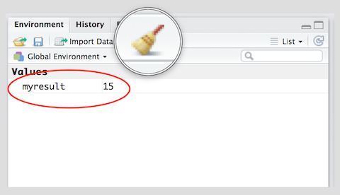
To delete all objects from the environment, you can use the broom button as shown in the picture above.
We called our object myresult but we can call it anything as long as we follow a few simple rules. Object names can contain upper or lower case letters (A-Z, a-z), numbers (0-9), underscores (_) or a dot (.) but all object names must start with a letter. Choose names that are descriptive and easy to type.
| Good Object Names | Bad Object Names |
|---|---|
| result | a |
| myresult | x1 |
| my.result | this.name.is.just.too.long |
| my_result | |
| data1 |
1.1.2.6 Sequences
We often need to create sequences when manipulating data. For instance, you might want to perform an operation on the first 10 rows of a dataset so we need a way to select the range we’re interested in.
There are two ways to create a sequence. Let’s try to create a sequence of numbers from 1 to 10 using the two methods:
- Using the colon
:operator. If you’re familiar with spreadsheets then you might’ve already used:to select cells, for exampleA1:A20. In R, you can use the:to create a sequence in a similar fashion:
[1] 1 2 3 4 5 6 7 8 9 10- Using the
seqfunction we get the exact same result:
[1] 1 2 3 4 5 6 7 8 9 10The seq function has a number of options which control how the sequence is generated. For example to create a sequence from 0 to 100 in increments of 5, we can use the optional by argument. Notice how we wrote by = 5 as the third argument. It is a common practice to specify the name of argument when the argument is optional. The arguments from and to are not optional, se we can write seq(0, 100, by = 5) instead of seq(from = 0, to = 100, by = 5). Both, are valid ways of achieving the same outcome. You can code whichever way you like. We recommend to write code such that you make it easy for your future self and others to read and understand the code.
 [1]   0   5  10  15  20  25  30  35  40  45  50  55  60  65  70  75  80  85
[19]  90  95 100
Another common use of the seq function is to create a sequence of a specific length. Here, we create a sequence from 0 to 100 with length 9, i.e., the result is a vector with 9 elements.
[1] 0.0 12.5 25.0 37.5 50.0 62.5 75.0 87.5 100.0Now it’s your turn:
- Create a sequence of odd numbers between 0 and 100 and save it in an object called
odd_numbers
- Next, display
odd_numberson the console to verify that you did it correctly
 [1]  1  3  5  7  9 11 13 15 17 19 21 23 25 27 29 31 33 35 37 39 41 43 45 47
[25] 49 51 53 55 57 59 61 63 65 67 69 71 73 75 77 79 81 83 85 87 89 91 93 95
[49] 97 99
What do the numbers in square brackets
[ ]mean? Look at the number of values displayed in each line to find out the answer.Use the
lengthfunction to find out how many values are in the objectodd_numbers.- HINT: Try
help(length)and look at the examples section at the end of the help screen.
- HINT: Try
[1] 501.1.2.7 Scripts
The Console is great for simple tasks but if you’re working on something consistently you would mostly likely want to save your work in some sort of a document or a file. Scripts in R are just plain text files that contain R code. You can edit a script just like you would edit a file in any word processing or note-taking application.
Create a new script using the menu or the toolbar button as shown below.
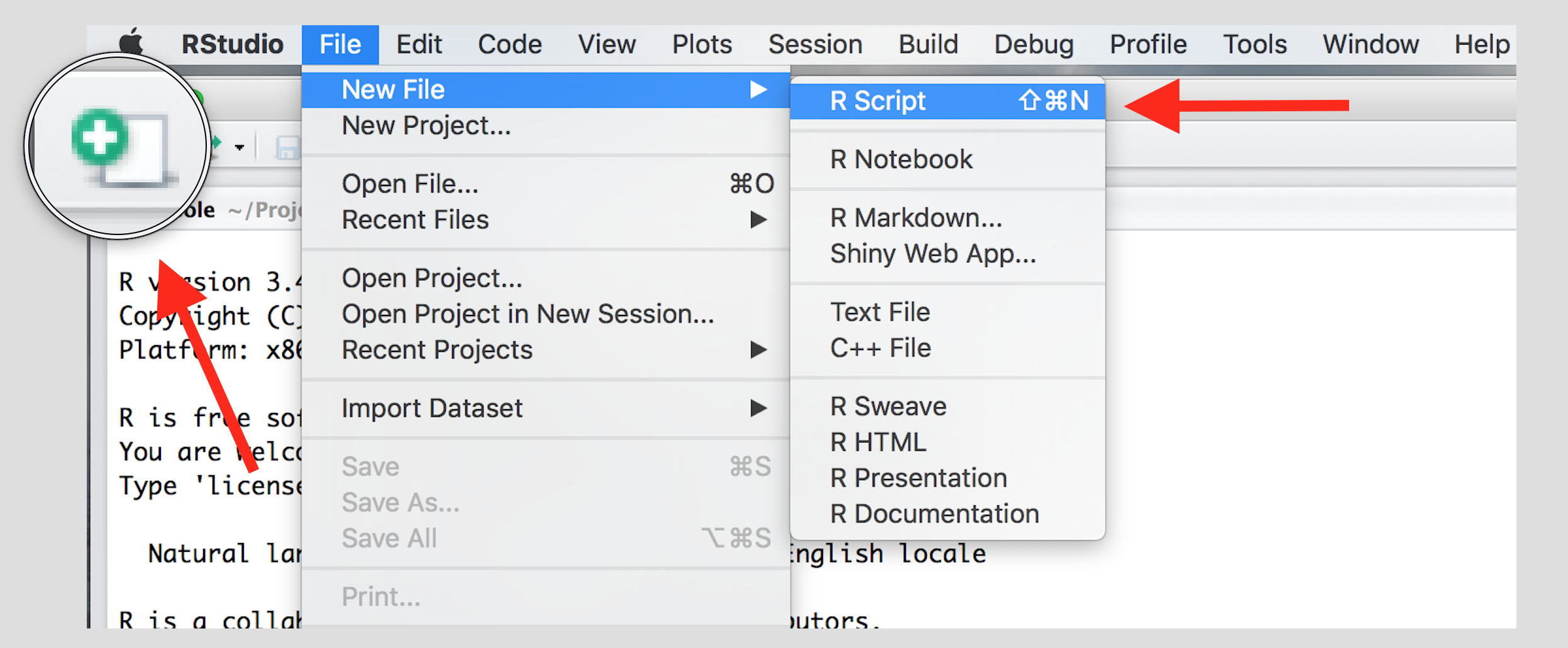
Once you’ve created a script, it is generally a good idea to give it a meaningful name and save it immediately. For our first session save your script as seminar1.R
| Familiarize yourself with the script window in RStudio, and especially the two buttons labeled Run and Source | 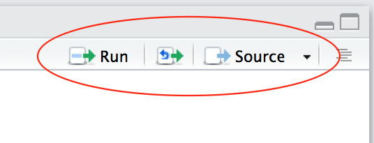 |
There are a few different ways to run your code from a script.
| One line at a time | Place the cursor on the line you want to run and hit CTRL-ENTER or use the Run button |
| Multiple lines | Select the lines you want to run and hit CTRL-ENTER or use the Run button |
| Entire script | Use the Source button |
1.1.2.8 Set up a project
When using scripts, the easiest way to work in R is through projects. Projects keep everything in the same place and make sure your code runs as it should. To set one up, you can simply follow the steps in this video:
You should see ‘Project: None’ in the top right hand corner of your screen. Click there.
Select ‘New Project…’
Select ‘New Directory’
Select ‘New Project’
Enter a sensible name in the ‘Directory name’ field (e.g. quants or polm083)
Select ‘Browse’
Choose a sensible location on your computer where you usually store your university work
Select ‘Create project’
This will create a folder in the location you chose, and inside that folder will be an R Project file. Save all your scripts and data in this folder. Whenever you start working in future sessions, make sure you open your project and work within it, rather than working aimlessly in RStudio. All your scripts and datsets will saved within this project and will be visible when you open the R-project.
Using scripts and organizing your scripts is an essential part of research as it means you can reproduce your research. When you publish your research you will be required to produce all the scripts and datasets to ensure reproducibility. You do not want to find you cannot remember what you have done after your paper has been accepted for publication!
1.1.3 Central Tendency
Central tendency is a way of understanding what is a typical value of a variable – what happens on average, or what we would expect to happen if we have no information to give us further clues. For example, what is the average age of people in the UK? Or, what level of education does the average UK citizen attain? Or, are there more men or women in the UK?
The appropriate measure of central tendency depends on the level of measurement of the variable: continuous, ordinal or nominal.
| Level of measurement | Appropriate measure of central tendency |
|---|---|
| Interval* | arithmetic mean (or average) |
| Ordinal | median (or the central observation) |
| Nominal | mode (the most frequent value) |
* Interval (sometimes called ‘quantitative’) variables are usually treated as continuous but can sometimes, strictly speaking, be discrete. In either case the mean tends to be an appropriate measure of central tendency. See page 26 of Statistical Methods for the Social Sciences by Alan Agresti.
1.1.3.1 Mean
Imagine eleven students take a statistics exam. We want to know about the central tendency of these grades. This is a continuous variable, so we want to calculate the mean. The mean is the arithmetic average: all of the results summed up, and divided by the number of results.
R is vectorised. This means that often, rather than dealing with individual values or data points, we deal with a series of data points that all belong to one ‘vector’ based on some connection. For example, we could create a vector of all the grades the students got in the exam. We create our vector of eleven (fake) grades using the c() function, where c stands for ‘collect’ or ‘concatenate’:
We can then do things to this vector as a whole, rather than to its individual components. R will do this automatically when we pass the vector to a function, because it is a vectorised coding language. All ‘vector’ means is a series of connected values like this. (A ‘list’ of values, if you like, but ‘list’ has a different, specific meaning in R, so we should really avoid that word here.)
We now take the sum of the grades.
We also take the number of grades
The mean is the sum of grades over the number of grades.
[1] 83.90909R provides us with an even easier way to do the same with a function called mean().
[1] 83.90909Remember that grades is an object we created by assigning the vector c(80, 90, 85, 71, 69, 85, 83, 88, 99, 81, 92) to the name ‘grades’ using the assignment operator <-.
1.1.3.2 Median
The median is the appropriate measure of central tendency for ordinal variables. Ordinal means that there is a rank ordering but not equally spaced intervals between values of the variable. Education is a common example. In education, more education is generally better. But the difference between primary school and secondary school is not the same as the difference between secondary school and an undergraduate degree. If you have only been to primary school, the difference between you and someone who has been to secondary school is probably going to be larger than the difference between someone who has been to secondary school and someone who has an undergraduate degree.
Let’s generate a fake example with 100 people. We use numbers to code different levels of education.
| Code | Meaning | Frequency in our data |
| 0 | no education | 1 |
| 1 | primary school | 5 |
| 2 | secondary school | 55 |
| 3 | undergraduate degree | 20 |
| 4 | postgraduate degree | 10 |
| 5 | doctorate | 9 |
We introduce a new function to create a vector. The function rep() replicates elements of a vector. Its arguments are the item x to be replicated and the number of times to replicate. Below, we create the variable education with the frequency of education level indicated above. Note that the arguments x = and times = do not have to be written out, but it is often a good idea to do this anyway, to make your code clear and unambiguous.
edu <- c( rep(x = 0, times = 1),
          rep(x = 1, times = 5),
          rep(x = 2, times = 55),
          rep(x = 3, times = 20),
          rep(4, 10), rep(5, 9)) # works without 'x =', 'times ='
The median level of education is the level where 50 percent of the observations have a lower or equal level of education and 50 percent have a higher or equal level of education. That means that the median splits the data in half.
We use the median() function for finding the median.
[1] 2The median level of education is secondary school.
1.1.3.3 Mode
The mode is the appropriate measure of central tendency if the level of measurement is nominal. It is the most common value. Nominal means that there is no ordering implicit in the values that a variable takes on. We create data from 1000 (fake) voters in the United Kingdom who each express their preference on remaining in or leaving the European Union. The options are leave or stay. Leaving is not greater than staying and vice versa (even though we all order the two options normatively).
| Code | Meaning | Frequency in our data |
| 0 | leave | 509 |
| 1 | stay | 491 |
The mode is the most common value in the data. There is no mode function in R. The most straightforward way to determine the mode is to use the table() function. It returns a frequency table. We can easily see the mode in the table. As your coding skills increase, you will see other ways of recovering the mode from a vector.
stay
  0   1
509 491
The mode is leaving the EU because the number of ‘leavers’ (0) is greater than the number of ‘remainers’ (1).
1.1.4 Dispersion
Central tendency is useful information, but two very different sets of data can have the same central tendency value while looking very different overall, because of different levels of dispersion. Dispersion describes how much variability around the central tendency there is in a variable or dataset.
The appropriate measure of dispersion again depends on the level of measurement of the variable we wish to describe.
| Level of measurement | Appropriate measure of dispersion |
|---|---|
| Interval* | variance and/or standard deviation |
| Ordinal | range or interquartile range |
| Nominal | proportion in each category |
* Interval (sometimes called ‘quantitative’) variables are usually treated as continuous but can sometimes, strictly speaking, be discrete. In either case the standard deviation tends to be an appropriate measure of central tendency. See page 26 of Statistical Methods for the Social Sciences by Alan Agresti.
1.1.4.1 Variance and standard deviation
Both the variance and the standard deviation tell us how much an average realisation of a variable differs from the mean of that variable. So, they essentially tell us how much, on average, our observations differ from the average observation.
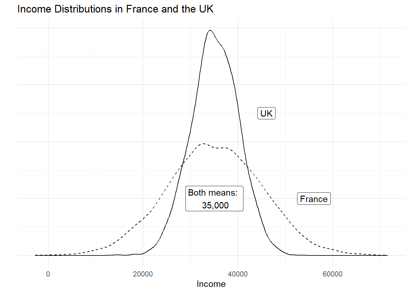
Let’s assume that our variable is income in the UK. Let’s assume that its mean is £35,000 per year. We also assume that the average deviation from £35,000 is £5,000. If we ask 100 people in the UK at random about their income, we get 100 different answers. If we average the differences betweeen the 100 answers and £35,000, we would get £5,000. Suppose that the average income in France is also £35,000 per year but the average deviation is £10,000 instead. This would imply that income is more equally distributed in the UK than in France, even though on average people earn around the same amount.
Dispersion is important to describe data, as this example illustrates. Although mean income in our hypothetical example is the same in France and the UK, the distribution is tighter in the UK. The figure below illustrates our example:
The variance gives us an idea about the variability of the data. The formula for the variance in the population is \[ \frac{\sum_{i=1}^n(x_i - \mu_x)^2}{n}\]
The formula for the variance in a sample adjusts for sampling variability, i.e., uncertainty about how well our sample reflects the population by subtracting 1 in the denominator. Subtracting 1 will have next to no effect if n is large but the effect increases the smaller \(n\) is. The smaller \(n\) is, the larger the sample variance. The intuition is, that in smaller samples, we are less certain that our sample reflects the population. We, therefore, adjust variability of the data upwards. The formula is
\[ \frac{\sum_{i=1}^n(x_i - \bar{x})^2}{n-1}\]
Notice the different notation for the mean in the two formulas. We write \(\mu_x\) for the mean of x in the population and \(\bar{x}\) for the mean of x in the sample. Notation is, however, unfortunately not always consistent.
Take a minute to consider the formula. There are four steps: (1) in the numerator - the top part, above the horizontal line - we subtract the mean of all the different values of x from each individual value of x. (2) We square each of the results of this. (3) We add up all these squared numbers. (4) We divide the result by the number of values (n) minus 1.
| Obs | Var | Dev. from mean | Squared dev. from mean |
|---|---|---|---|
| i | grade | \(x_i-\bar{x}\) | \((x_i-\bar{x})^2\) |
| 1 | 80 | -3.9090909 | 15.2809917 |
| 2 | 90 | 6.0909091 | 37.0991736 |
| 3 | 85 | 1.0909091 | 1.1900826 |
| 4 | 71 | -12.9090909 | 166.6446281 |
| 5 | 69 | -14.9090909 | 222.2809917 |
| 6 | 85 | 1.0909091 | 1.1900826 |
| 7 | 83 | -0.9090909 | 0.8264463 |
| 8 | 88 | 4.0909091 | 16.7355372 |
| 9 | 99 | 15.0909091 | 227.7355372 |
| 10 | 81 | -2.9090909 | 8.4628099 |
| 11 | 92 | 8.0909091 | 65.4628099 |
| \(\sum_{i=1}^n\) | 762.9090909 | ||
| \(\div n-1\) | 76.2909091 | ||
| \(\sqrt{}\) | 8.7344667 |
Our first grade (80) is below the mean (83.9090909). The result of \(x_i - \bar{x}\) is, thus, negative. Our second grade (90) is above the mean, so that the result of \(x_i - \bar{x}\) is positive. Both are deviations from the mean (think of them as distances). Our sum shall reflect the total sum of these distances, which need to be positive. Hence, we square these distances from the mean. Recall that any number, multiplied by itself (i.e. squared) results in a positive number – even when the original number is negative. Having done this for all eleven observations, we sum the squared distances. Dividing by 10 (with the sample adjustment), gives us the average squared deviation. This is the variance, or the average sum of squares. The units of the variance — squared deviations — are somewhat awkward. We return to this in a moment.
With R at our disposal, we have no need to carry out these cumbersome calculations. We simply take the variance in R by using the var() function. By default var() takes the sample variance.
[1] 76.29091The average squared difference form our mean grade is 76.2909091. But what does that mean? We would like to get rid of the square in our units. That’s what the standard deviation does. The standard deviation is the square root of the variance.
\[ \sqrt{\frac{\sum_{i=1}^n(x_i - \bar{x})^2}{n-1}}\]
Note that this formula is, accordingly, just the variance formula above, all within a square root. Again, this is made very simple by R. We get this standard deviation — that is, the average deviation from our mean grade (83.9090909) — with the sd() function.
[1] 8.734467The standard deviation is much more intuitive than the variance because its units are the same as the units of the variable we are interested in. “Why teach us about this awful variance then?”, you ask. Mathematically, we have to compute the variance before getting the standard deviation. We recommend that you use the standard deviation to describe the variability of your continuous data.
Note: We used the sample variance and sample standard deviation formulas. If the eleven assignments represent the population, we would use the population variance formula. Whether the 11 cases represent a sample or the population depends on what we want to know. If we want learn about all students’ assignments or future assignments, the 11 cases are a sample.
1.1.4.2 Range and interquartile range
The proper measure of dispersion of an ordinal variable is the range or the interquartile range. The interquartile range is usually the preferred measure because the range is strongly affected by outlying cases.
Let’s take the range first. We get back to our education example. In R, we use the range() function to compute the range.
[1] 0 5Our data ranges from no education all the way to those with a doctorate. However, no education is not a common value. Only one person in our sample did not have any education. The interquartile range is the range from the 25th to the 75th percentiles, i.e., it contains the central 50 percent of the distribution.
The 25th percentile is the value of education that 25 percent or fewer people have (when we order education from lowest to highest). We use the quantile() function in R to get percentiles. The function takes two arguments: x is the data vector and probs is the percentile.
25%
2 75%
3 Therefore, the interquartile range is from 2, secondary school to 3, undergraduate degree.
1.1.4.3 Proportion in each category
To describe the distribution of our nominal variable, support for remaining in the European Union, we use the proportions in each category.
Recall, that we looked at the frequency table to determine the mode:
stay
  0   1
509 491
To get the proportions in each category, we divide the values in the table, i.e., 509 and 491, by the sum of the table, i.e., 1000.
stay
    0     1
0.509 0.491
# `R` also has a built in function for this, simply pass the table to `prop.table()`
prop.table(table(stay))stay
0 1
0.509 0.491 1.1.5 Homework exercises
- Create a script and call it assignment01. Save your script.
- Download this cheat-sheet and go over it. You won’t understand most of it right away. But it will become a useful resource. Look at it often.
- Calculate the square root of 1369 using the
sqrt()function. - Square the number 13 using the
^operator. - What is the result of summing all numbers from 1 to 100?
We take a sample of yearly income in London. The values that we got are: 19395, 22698, 40587, 25705, 26292, 42150, 29609, 12349, 18131, 20543, 37240, 28598, 29007, 26106, 19441, 42869, 29978, 5333, 32013, 20272, 14321, 22820, 14739, 17711, 18749.
- Create the variable
incomewith the values from our fake London sample in R. - Describe London income using the appropriate measures of central tendency and dispersion.
- Compute the standard deviation without using the
sd()function.
For each of these incomes, we also find out if that person is married or not. The responses show that there are 16 married people and 9 unmarried people.
- Create the variable
marriedwith the values from our fake sample. Therep()function used above might be useful. - Describe the marriage status of our sample using appropriate measures of central tendency and dispersion.
Finally, we also find out these people’s highest completed level of education, where 1 = secondary school, 2 = undergraduate, and 3 = postgraduate. The values are: 3, 3, 3, 2, 3, 2, 2, 2, 3, 1, 2, 2, 1, 2, 3, 1, 3, 3, 1, 1, 1, 1, 3, 2, 3.
Create the variable
educationwith the values from our fake sample.Describe the education status of our fake sample using appropriate measures of central tendency and dispersion.
Save your script, which should now include the answers to all the exercises.