2.2 Solutions

2.2.0.1 Exercise 1

Load the quality of government dataset.

qog <- read.csv("https://raw.githubusercontent.com/QMUL-SPIR/Public_files/master/datasets/QoG2012.csv")

2.2.0.2 Exercise 2

Rename the variable wdi_gdpc to gdpc using rename() from the tidyverse.

library(tidyverse)

qog <- rename(qog, gdpc = wdi_gdpc)

2.2.0.3 Exercise 3

Delete all rows with missing values on gdpc.

qog <- drop_na(qog, gdpc)

2.2.0.4 Exercise 4

Inspect former_col and delete rows with missing values on it.

# we instpect the variable and check for missings
summary(qog$former_col)

   Min. 1st Qu.  Median    Mean 3rd Qu.    Max. 
 0.0000  0.0000  1.0000  0.6348  1.0000  1.0000

# no missing data!

2.2.0.5 Exercise 5

Turn former_col into a factor variable with appropriate labels.

# we check the current data type
str(qog$former_col)

 int [1:178] 0 0 1 1 1 0 1 0 0 1 ...

# it's numeric (or 'integer'), so we change it to nominal
qog$former_col <- factor(qog$former_col,
                         levels = c(0,1),
                         labels = c("not colonised", "former colony" ))

# let's check the results
table(qog$former_col)


not colonised former colony 
           65           113

2.2.0.6 Exercise 6

Subset the dataset so that it only has the gdpc, undp_hdi, and former_col variables.

qog <- select(
  qog,
  gdpc,
  undp_hdi,
  former_col)

2.2.0.7 Exercise 7

Plot the distribution of gdpc conditional on former colony status, using theme_minimal(), labs() and scale_colour_discrete() to make sure your plot is clear and easy to understand.

gg_gdpc <- ggplot(data = qog, 
                  mapping = aes(gdpc, 
                                group = former_col,
                                colour = former_col)) + 
  geom_density() + 
  labs(x = "GDP per capita", # clearer x axis label
       y = "Density", # clearer y axis label
       title = "Distribution of GDP conditional on former colony status") + # clearer title 
  scale_color_discrete(name = "Former colony", # change legend title
                       labels = c("Never colonised", # change legend labels
                                  "Colonised")) +
  theme_minimal()

gg_gdpc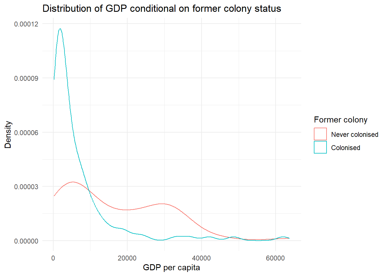

2.2.0.8 Exercise 8

Compute the probability that a country is richer than 55,000 per capita.

# get the empirical cumulative distribution of wealth
dist_wealth <- ecdf(qog$gdpc)

# probability
1 - dist_wealth(55000)

[1] 0.01123596

The probability is 0.01. Put differently 1 percent of countries are richer than 55,000 US dollars per capita.

2.2.0.9 Exercise 9

Compute the conditional expectation of wealth for a country that is not a former colony.

The conditional expectation is the mean of wealth among all former colonies.

# dataset of just non-former colonies
non_colonies <- filter(qog, 
                       former_col == "not colonised")

# take mean of gdp
mean(non_colonies$gdpc)

[1] 16415.39

The conditional expectation of wealth for non-former colonies is approximately 16415 US dollars per capita.

2.2.0.10 Exercise 10

What is the probability that a former colony is 2 standard deviations below the mean wealth level?

We first find out what the standard deviation and mean of wealth are in the conditional distribution of wealth for former colonies.

# dataset of just former colonies
colonies <- filter(qog, former_col == "former colony")

# standard deviation of wealth for former colonies
sd_wealth_cols <- sd(colonies$gdpc)
sd_wealth_cols

[1] 9783.914

# but what is the mean?
mean_wealth_cols <- mean(colonies$gdpc)
mean_wealth_cols

[1] 6599.714

The standard deviation is greater than the mean. Apparently, former colonies are very different. Some do poorly and some extremely well. Negative wealth does not exist. Consequently, the answer is that there is 0 probability of a country having a gdp two standard deviations below the mean.

2.2.0.11 Exercise 11

Compute the probability that any country is the wealth interval from 20,000 to 50,000.

We compute the cumulative probabilities that a country has 20,000 and 50,000 and then take the difference.

# get the empirical cumulative distribution of wealth
dist_wealth_2 <- ecdf(qog$gdpc)

# cumulative probability of 20,000
p1 <- dist_wealth_2(20000)
# cumulative probability of 50,000
p2 <- dist_wealth_2(50000)
# probability of country in the interval
p2 - p1

[1] 0.1741573

The probability is approximately 0.17, so we expect about 17% of countries to fall in this interval.