2.2 Solutions

# if tidyverse not already installed
install.packages("tidyverse")

library(tidyverse)

2.2.1 Exercise 1

Use the names() function to display the variable names of the longley dataset.

names(longley)

[1] "GNP.deflator" "GNP"          "Unemployed"   "Armed.Forces" "Population"  
[6] "Year"         "Employed"    

2.2.2 Exercise 2

Use square brackets to access the 4th column of the dataset.

longley[, 4]

 [1] 159.0 145.6 161.6 165.0 309.9 359.4 354.7 335.0 304.8 285.7 279.8 263.7
[13] 255.2 251.4 257.2 282.7

2.2.3 Exercise 3

Use the dollar sign to access the 4th column of the dataset.

longley$Armed.Forces

 [1] 159.0 145.6 161.6 165.0 309.9 359.4 354.7 335.0 304.8 285.7 279.8 263.7
[13] 255.2 251.4 257.2 282.7

Note: There is yet another way to access the 4th column of the dataset. We can put the variable name into the square brackets using quotes like so:

longley[, "Armed.Forces"]

 [1] 159.0 145.6 161.6 165.0 309.9 359.4 354.7 335.0 304.8 285.7 279.8 263.7
[13] 255.2 251.4 257.2 282.7

2.2.4 Exercise 4

Access the two cells from row 4 and column 1 and row 6 and column 3.

# row 4, column 1
longley[4, 1]

[1] 89.5

# row 6, column 3
longley[6, 3]

[1] 193.2

2.2.5 Exercise 5

Using the longley data produce a line plot with GNP on the y-axis and population on the x-axis.

g_e5 <- ggplot(longley, aes(Population, GNP)) +
  geom_line() +
  theme_minimal() +
  ggtitle("Relationship of Population Size and Size of the Economy")

g_e5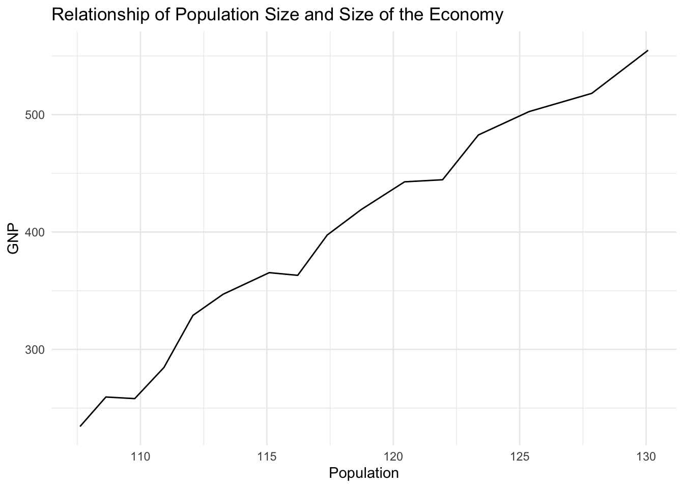

2.2.6 Exercise 6

Use the labs() function to change the axis labels to “Population older than 14 years of age” and “Gross national product”.

g_e6 <- ggplot(longley, aes(Population, GNP)) +
  geom_line() +
  theme_minimal() +
  ggtitle("Relationship of Population Size and Size of the Economy") +
  xlab("Population older than 14 years of age") +
  ylab("Gross national product")

g_e6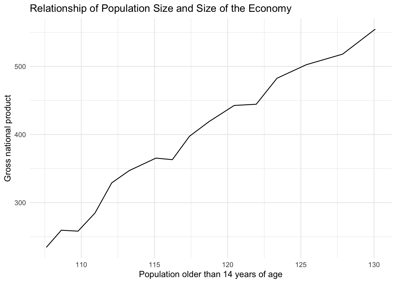

2.2.7 Exercise 7

Create a boxplot showing the distribution of IMMBRIT by each party in the data and plot these in one plot next to each other.

To do that, we load the non-western foreigners dataset first.

Note: You have to set your working directory that R operates in to the location of the dataset.

# load perception of non-western foreigners data
load("BSAS_manip.RData")

We have five parties in our dataset. We plot 5 boxplots next to each other. Hence, we separate the plot window into 1 row and 5 columns.

# create Tory/Labour indicator 
data2$party <- case_when(
  data2$Cons == 1 ~ "Con", # are they Conservative
  data2$Lab == 1 ~ "Lab", # are they Labour
  data2$SNP == 1 ~ "SNP", # are they SNP
  data2$Ukip == 1 ~ "Ukip", # are they UKIP
  data2$BNP == 1 ~ "BNP", # are they BNP
  TRUE ~ "Other") # are they neither


# plot

g5 <- ggplot(data2, aes(y = IMMBRIT)) +
  geom_boxplot() +
  labs(y = "Subjective number of immigrants per 100 British",
       title = "Perception of Immigration from Non-Western Countries, among Conservatives and Labour") +
  theme_minimal() + 
  facet_grid(~ party)

g5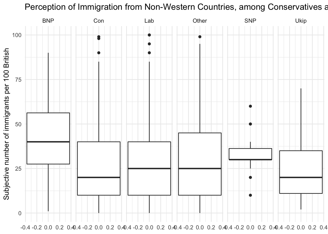 

2.2.8 Exercises 8 and 9

We combine the answer to questions 9 and 10.

Question 9: Is there a difference between women and men in terms of their subjective estimation of foreigners?

Question 10: What is the difference between women and men?

Women’s subjective estimate is the mean of IMMBRIT across women and equally, men’s subjective estimate is the mean of IMMBRIT over all men. Let’s get these numbers by filtering the dataset and using the mean function.

women_bsas <- filter(data2, RSex == 2) # filter dataset to include only women
women_mean <- mean(women_bsas$IMMBRIT) # get mean of immbrit column
women_mean

[1] 32.79159

men_bsas <- filter(data2, RSex == 1) # filter dataset to include only men
men_mean <- mean(men_bsas$IMMBRIT) # get mean of immbrit column
men_mean

[1] 24.53766

The difference between women and men is the difference in means. Let’s take the difference between them. The difference in means is often referred to as the first difference.

first_difference <- women_mean - men_mean
first_difference

[1] 8.253937

Let’s round that number. We don’t like to see so many decimal places. You should usually present precision up to the second decimal place. We can use the round() function. The first argument is number to round and the second is the amount of digits.

round(first_difference, 2)

[1] 8.25

We do find a difference between men and women. On average, women’s estimate of the number of non-western foreingers is 8.25 greater than men’s estimate.

At this point we have established that there is a difference in our sample. Samples are subject to sampling variability. That means, we cannot yet say that the difference is systematic, i.e., British women, generally, think that there are more non-western foreingers than British men.