Chapter 1 Introduction to R and data manipulation
1.1 Seminar
In this seminar session, we introduce working with R. We illustrate some basic functionality and help you familiarise yourself with the look and feel of RStudio. Measures of central tendency and dispersion are easy to calculate in R. We focus on introducing the logic of R first and then describe how central tendency and dispersion are calculated in the end of the seminar.
1.1.1 Getting Started
Install R and RStudio on your computer by downloading them from the following sources:
- Download R from The Comprehensive R Archive Network (CRAN)
- Download RStudio from RStudio.com
1.1.2 RStudio
Let’s get acquainted with R. When you start RStudio for the first time, you’ll see three panes:
1.1.3 Console
The Console in RStudio is the simplest way to interact with R. You can type some code at the Console and when you press ENTER, R will run that code. Depending on what you type, you may see some output in the Console or if you make a mistake, you may get a warning or an error message.
Let’s familiarize ourselves with the console by using R as a simple calculator:
2 + 4[1] 6Now that we know how to use the + sign for addition, let’s try some other mathematical operations such as subtraction (-), multiplication (*), and division (/).
10 - 4[1] 65 * 3[1] 157 / 2[1] 3.5| You can use the cursor or arrow keys on your keyboard to edit your code at the console: - Use the UP and DOWN keys to re-run something without typing it again - Use the LEFT and RIGHT keys to edit |
 |
Take a few minutes to play around at the console and try different things out. Don’t worry if you make a mistake, you can’t break anything easily!
1.1.4 Functions
Functions are a set of instructions that carry out a specific task. Functions often require some input and generate some output. For example, instead of using the + operator for addition, we can use the sum function to add two or more numbers.
sum(1, 4, 10)[1] 15In the example above, 1, 4, 10 are the inputs and 15 is the output. A function always requires the use of parenthesis or round brackets (). Inputs to the function are called arguments and go inside the brackets. The output of a function is displayed on the screen but we can also have the option of saving the result of the output. More on this later.
1.1.5 Getting Help
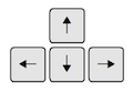
Another useful function in R is help which we can use to display online documentation. For example, if we wanted to know how to use the sum function, we could type help(sum) and look at the online documentation.
help(sum)The question mark ? can also be used as a shortcut to access online help.
?sum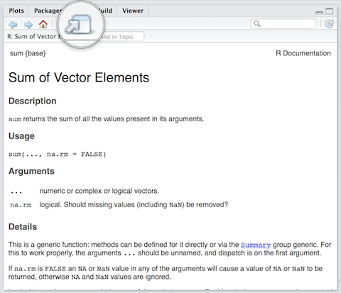
Use the toolbar button shown in the picture above to expand and display the help in a new window.
Help pages for functions in R follow a consistent layout generally include these sections:
| Description | A brief description of the function |
| Usage | The complete syntax or grammar including all arguments (inputs) |
| Arguments | Explanation of each argument |
| Details | Any relevant details about the function and its arguments |
| Value | The output value of the function |
| Examples | Example of how to use the function |
1.1.6 The Assignment Operator
Now we know how to provide inputs to a function using parenthesis or round brackets (), but what about the output of a function?
We use the assignment operator <- for creating or updating objects. If we wanted to save the result of adding sum(1, 4, 10), we would do the following:
myresult <- sum(1, 4, 10)The line above creates a new object called myresult in our environment and saves the result of the sum(1, 4, 10) in it. To see what’s in myresult, just type it at the console:
myresult[1] 15Take a look at the Environment pane in RStudio and you’ll see myresult there.
To delete all objects from the environment, you can use the broom button as shown in the picture above.
We called our object myresult but we can call it anything as long as we follow a few simple rules. Object names can contain upper or lower case letters (A-Z, a-z), numbers (0-9), underscores (_) or a dot (.) but all object names must start with a letter. Choose names that are descriptive and easy to type.
| Good Object Names | Bad Object Names |
|---|---|
| result | a |
| myresult | x1 |
| my.result | this.name.is.just.too.long |
| my_result | |
| data1 |
1.1.7 Sequences
We often need to create sequences when manipulating data. For instance, you might want to perform an operation on the first 10 rows of a dataset so we need a way to select the range we’re interested in.
There are two ways to create a sequence. Let’s try to create a sequence of numbers from 1 to 10 using the two methods:
- Using the colon
:operator. If you’re familiar with spreadsheets then you might’ve already used:to select cells, for exampleA1:A20. In R, you can use the:to create a sequence in a similar fashion:
1:10 [1] 1 2 3 4 5 6 7 8 9 10- Using the
seqfunction we get the exact same result:
seq(from = 1, to = 10) [1] 1 2 3 4 5 6 7 8 9 10The seq function has a number of options which control how the sequence is generated. For example to create a sequence from 0 to 100 in increments of 5, we can use the optional by argument. Notice how we wrote by = 5 as the third argument. It is a common practice to specify the name of argument when the argument is optional. The arguments from and to are not optional, se we can write seq(0, 100, by = 5) instead of seq(from = 0, to = 100, by = 5). Both, are valid ways of achieving the same outcome. You can code whichever way you like. We recommend to write code such that you make it easy for your future self and others to read and understand the code.
seq(from = 0, to = 100, by = 5) [1] 0 5 10 15 20 25 30 35 40 45 50 55 60 65 70 75 80 85 90
[20] 95 100Another common use of the seq function is to create a sequence of a specific length. Here, we create a sequence from 0 to 100 with length 9, i.e., the result is a vector with 9 elements.
seq(from = 0, to = 100, length.out = 9)[1] 0.0 12.5 25.0 37.5 50.0 62.5 75.0 87.5 100.0Now it’s your turn:
- Create a sequence of odd numbers between 0 and 100 and save it in an object called
odd_numbers
odd_numbers <- seq(1, 100, 2)- Next, display
odd_numberson the console to verify that you did it correctly
odd_numbers [1] 1 3 5 7 9 11 13 15 17 19 21 23 25 27 29 31 33 35 37 39 41 43 45 47 49
[26] 51 53 55 57 59 61 63 65 67 69 71 73 75 77 79 81 83 85 87 89 91 93 95 97 99What do the numbers in square brackets
[ ]mean? Look at the number of values displayed in each line to find out the answer.- Use the
lengthfunction to find out how many values are in the objectodd_numbers.- HINT: Try
help(length)and look at the examples section at the end of the help screen.
- HINT: Try
length(odd_numbers)[1] 501.1.8 Scripts
The Console is great for simple tasks but if you’re working on a project you would mostly likely want to save your work in some sort of a document or a file. Scripts in R are just plain text files that contain R code. You can edit a script just like you would edit a file in any word processing or note-taking application.
Create a new script using the menu or the toolbar button as shown below.
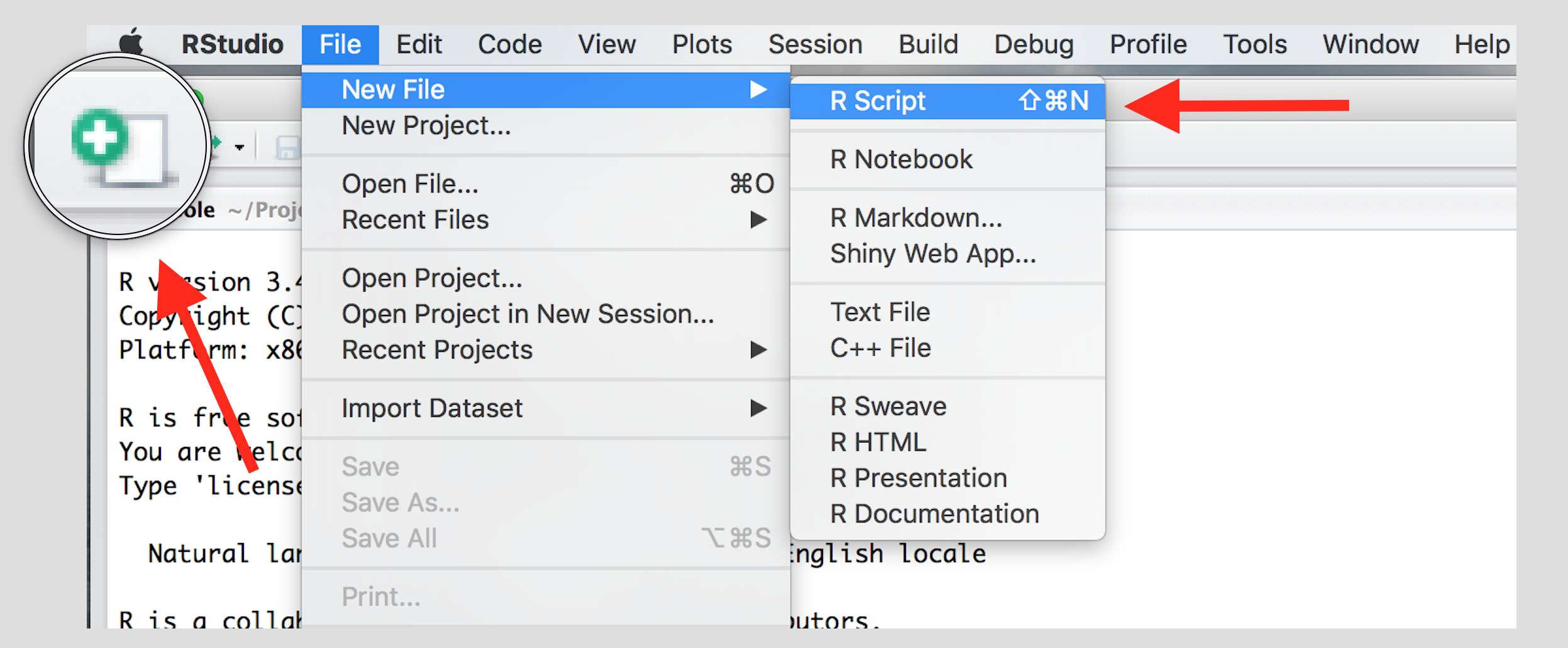
Once you’ve created a script, it is generally a good idea to give it a meaningful name and save it immediately. For our first session save your script as seminar1.R
| Familiarize yourself with the script window in RStudio, and especially the two buttons labeled Run and Source | 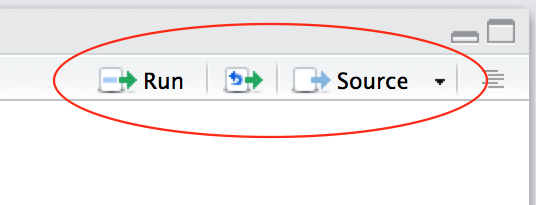 |
There are a few different ways to run your code from a script.
| One line at a time | Place the cursor on the line you want to run and hit CTRL-ENTER or use the Run button |
| Multiple lines | Select the lines you want to run and hit CTRL-ENTER or use the Run button |
| Entire script | Use the Source button |
1.1.9 Working with Data
In the previous section, R may have seemed fairly labour-intensive. We had to enter all our data manually and each line of code had to be written into the command line. Fortunately this isn’t routinely the case, as we can use scripts to keep track of our code. Type the following into the script:
#This is my first R script
My.Data<- data.frame(0:10, 20:30)
print(My.Data)
X0.10 X20.30
1 0 20
2 1 21
3 2 22
4 3 23
5 4 24
6 5 25
7 6 26
8 7 27
9 8 28
10 9 29
11 10 30In the script window, if you highlight all the code you have written and press the “Run” button on the top on the scripting window you will see that the code is sent to the command line and the text on the line after the # (known as a ‘comment’) is ignored. From now on, to run a command, type your code in the script window, ensure the cursor is on the correct line and press CTRL + ENTER or use the Run button. If you have an error, edit the line in the script and run the code again. The My.Data object is a data frame in need of some sensible column headings. You can add these by typing:
#Add column names
colnames(My.Data)<- c("X", "Y")

#Print My.Data object to check names were added successfully
print(My.Data)
X Y
1 0 20
2 1 21
3 2 22
4 3 23
5 4 24
6 5 25
7 6 26
8 7 27
9 8 28
10 9 29
11 10 30#You can also print by just typing the object name
My.Data X Y
1 0 20
2 1 21
3 2 22
4 3 23
5 4 24
6 5 25
7 6 26
8 7 27
9 8 28
10 9 29
11 10 30Until now we have generated the data used in the examples above. One of R’s great strengths is its ability to load in data from almost any file format. Comma Separated Value (CSV) files are our preferred choice. These can be thought of as stripped down Excel spreadsheets. They are an extremely simple format so they are easily machine readable and can therefore be easily read in and written out of R. Since we are now reading and writing files it is good practice to tell R what your working directory is.
The working directory is the folder on the computer where you wish to store the data files you are working with. You can create a folder called “POL252” for example. If you are using RStudio, on the lower right of the screen is a window with a “Files” tab. If you click on this tab you can then navigate to the folder you wish to use. You can then click on the “More” button and then “Set as Working Directory”. You should then see some code similar to the below appear in the command line. It is also possible to type the code in manually.
#Set the working directory. The bit between the "" needs to specify the path to the folder you wish to use (you will see my file path below).  You may need to create the folder first.

setwd("~/POL252") # Note the single / (\\ will also work).
Note that, as we are mostly using RStudio Cloud on this course, there shouldn’t be any need to set a working directory. Instead, each week automatically has its own project directory which you will access when working on the relevant seminar. This is still worth knowing, though, as if you use R beyond this module then you will likely want the RStudio programme installed directly on your computer, in which case you’ll need to get to grips with working directories.
One way of opening data is by using the read.csv() function. The file can be saved in your computer (preferably in your working directory), in your RStudio Cloud project directory, or even online on a separate website. When we want to download a data file from a website, we need to add the url between quotation marks (“”). We are going to load a dataset that shows London’s historic population for each of its Boroughs.
#Load a dataset in a csv file
pop <- read.csv("https://data.london.gov.uk/download/historic-census-population/2c7867e5-3682-4fdd-8b9d-c63e289b92a6/census-historic-population-borough.csv")
To view the object type, we use:
class(pop)[1] "data.frame"We now know that the type is data frame, which will have implications for our future seminars. We can also look at the contents of the object. Data frames can be too large to show in the console, so we usually look at the beginning of the dataset - head() - or the end - tail().
head(pop) Area.Code Area.Name Persons.1801 Persons.1811 Persons.1821
1 00AA City of London 129000 121000 125000
2 00AB Barking and Dagenham 3000 4000 5000
3 00AC Barnet 8000 9000 11000
4 00AD Bexley 5000 6000 7000
5 00AE Brent 2000 2000 3000
6 00AF Bromley 8000 9000 11000
Persons.1831 Persons.1841 Persons.1851 Persons.1861 Persons.1871 Persons.1881
1 123000 124000 128000 112000 75000 51000
2 6000 7000 8000 8000 10000 13000
3 13000 14000 15000 20000 29000 41000
4 9000 11000 12000 15000 22000 29000
5 3000 5000 5000 6000 19000 31000
6 12000 14000 16000 22000 42000 62000
Persons.1891 Persons.1901 Persons.1911 Persons.1921 Persons.1931 Persons.1939
1 38000 27000 20000 14000 11000 9000
2 19000 27000 39000 44000 138000 184000
3 58000 76000 118000 147000 231000 296000
4 37000 54000 60000 76000 95000 179000
5 65000 120000 166000 184000 251000 310000
6 83000 100000 116000 127000 165000 237000
Persons.1951 Persons.1961 Persons.1971 Persons.1981 Persons.1991 Persons.2001
1 5000 4767 4000 5864 4230 7181
2 189000 177092 161000 149786 140728 163944
3 320000 318373 307000 293436 284106 314565
4 205000 209893 217000 215233 211404 218301
5 311000 295893 281000 253275 227903 263466
6 268000 294440 305000 296539 282920 295535
Persons.2011
1 7375
2 185911
3 356386
4 231997
5 311215
6 309392tail(pop) Area.Code Area.Name Persons.1801 Persons.1811 Persons.1821 Persons.1831
31 00BH Waltham Forest 8000 9000 11000 11000
32 00BJ Wandsworth 13000 16000 19000 23000
33 00BK Westminster 231000 254000 298000 354000
34 UKI1 Inner London 939000 1109000 1349000 1624000
35 UKI2 Outer London 162000 193000 224000 256000
36 H Greater London 1097000 1303000 1573000 1878000
Persons.1841 Persons.1851 Persons.1861 Persons.1871 Persons.1881
31 12000 13000 17000 28000 54000
32 28000 36000 52000 99000 173000
33 402000 462000 512000 524000 513000
34 1904000 2308000 2745000 3244000 3906000
35 302000 342000 445000 602000 817000
36 2207000 2651000 3188000 3841000 4713000
Persons.1891 Persons.1901 Persons.1911 Persons.1921 Persons.1931
31 112000 198000 258000 267000 283000
32 251000 319000 369000 380000 388000
33 481000 460000 421000 390000 372000
34 4432000 4898000 5002000 4978000 4898000
35 1142000 1609000 2160000 2408000 3213000
36 5572000 6510000 7162000 7387000 8110000
Persons.1939 Persons.1951 Persons.1961 Persons.1971 Persons.1981
31 286000 275000 248591 235000 215947
32 358000 331000 335451 302000 254898
33 347000 300000 271703 240000 191098
34 4441000 3680000 3492881 3031000 2497978
35 4176000 4513000 4504213 4422000 4215187
36 8615000 8197000 7997094 7452000 6713165
Persons.1991 Persons.2001 Persons.2011
31 203343 218335 258249
32 239162 260379 306995
33 177743 181284 219396
34 2343133 2766065 3231901
35 4050435 4405992 4942040
36 6393568 7172057 8173941To get to know a bit more about the file you have loaded R has a number of useful functions. We can use these to find out how many columns (variables) and rows (cases) the data frame (dataset) contains.
#Get the number of columns

ncol(pop)
[1] 24#Get the number of rows
nrow(pop)[1] 36#List the column headings
names(pop) [1] "Area.Code" "Area.Name" "Persons.1801" "Persons.1811" "Persons.1821"
[6] "Persons.1831" "Persons.1841" "Persons.1851" "Persons.1861" "Persons.1871"
[11] "Persons.1881" "Persons.1891" "Persons.1901" "Persons.1911" "Persons.1921"
[16] "Persons.1931" "Persons.1939" "Persons.1951" "Persons.1961" "Persons.1971"
[21] "Persons.1981" "Persons.1991" "Persons.2001" "Persons.2011"Given the number of columns in the pop data frame, subsetting by selecting on the columns of interest would make it easier to handle. In R there are two ways of doing this. The first uses the $ symbol to select columns by name and then create a new data frame object.
#Select the columns containing the Borough names and the 2011 population

pop.2011<- data.frame(pop$Area.Name, pop$Persons.2011)


head(pop.2011)
pop.Area.Name pop.Persons.2011
1 City of London 7375
2 Barking and Dagenham 185911
3 Barnet 356386
4 Bexley 231997
5 Brent 311215
6 Bromley 309392A second approach to selecting particular data is to use [Row, Column].
#Select the 1st row of the second column

pop[1,2]
[1] City of London
36 Levels: Barking and Dagenham Barnet Bexley Brent Bromley ... Westminster#Select the first 5 rows of the second column
pop[1:5,1][1] 00AA 00AB 00AC 00AD 00AE
36 Levels: 00AA 00AB 00AC 00AD 00AE 00AF 00AG 00AH 00AJ 00AK 00AL 00AM ... UKI2#Select the first 5 rows of columns 8 to 11
pop[1:5, 8:11] Persons.1851 Persons.1861 Persons.1871 Persons.1881
1 128000 112000 75000 51000
2 8000 8000 10000 13000
3 15000 20000 29000 41000
4 12000 15000 22000 29000
5 5000 6000 19000 31000#Assign the previous selection to a new object
pop.subset <- pop[1:5, 8:11]In the code snippet, note how the colon : is used to specify a range of values. We used the same technique to create the My.Data object above. The abilty to select particular columns means we can see how the population of London’s Boroughs have changed over the past century.
# Within the brackets you can add additional columns to the data frame so long as they are separated by commas

PopChange <- data.frame(pop$Area.Name, pop$Persons.2011-pop$Persons.1911)
If you type head(PopChange) you will see that the population change column (created to the right of the comma above) has a very long name. This can be changed using the names(), or colnamnes(), function
colnames(PopChange)<- c("Borough", "Change_1911_2011")Since we have done some new analysis and created additional information it would be good to save the PopChange object to our working directory. This is done using the code below. Within the brackets we put the name of the R object we wish to save on the left of the comma and the file name on the right of the comma (this needs to be in inverted commas). Remember to put “.csv” after since this is the file format we are saving in.
write.csv(PopChange, "Population_Change_1911_2011.csv")1.1.10 Exercises
- Create a script and call it assignment01. Save your script.
- Download this cheat-sheet and go over it. You won’t understand most of it right a away. But it will become a useful resource. Look at it often.
- Calculate the square root of 1369 using the
sqrt()function. - Square the number 13 using the
^operator. What is the result of summing all numbers from 1 to 100?
Using the London borough data, create a CSV file that contains the following columns:
The names of the London Boroughs
Population change between 1811 and 1911
Population change between 1911 and 1961
Population change 1961 and 2011
Which Boroughs had the most population growth during the 19th Century, and which had the slowest?
You may have noticed that there is an additional column in the pop data frame called Borough-Type. This indicates if a Borough is in inner (1) or outer (2) London. Is this variable ordinal or nominal?
Save your R script by pressing the Save button in the script window.